不同核的先验和后验高斯过程的说明

这个例子说明了一个的先验和先验 GaussianProcessRegressor 有不同的果仁。显示先验和后验分布的平均值、标准差和5个样本。

在这里，我们只给出一些例子。要了解更多关于核函数公式的信息，请参阅 User Guide .

# Authors: The scikit-learn developers
# SPDX-License-Identifier: BSD-3-Clause

Helper函数

在介绍每个可用于高斯过程的内核之前，我们将定义一个帮助函数，允许我们绘制从高斯过程中提取的样本。

此函数将采用 GaussianProcessRegressor 模型并将从高斯过程中提取样本。如果模型不匹配，则从先验分布中提取样本，而模型匹配后，则从后验分布中提取样本。

import matplotlib.pyplot as plt
import numpy as np


def plot_gpr_samples(gpr_model, n_samples, ax):
    """Plot samples drawn from the Gaussian process model.

    If the Gaussian process model is not trained then the drawn samples are
    drawn from the prior distribution. Otherwise, the samples are drawn from
    the posterior distribution. Be aware that a sample here corresponds to a
    function.

    Parameters
    ----------
    gpr_model : `GaussianProcessRegressor`
        A :class:`~sklearn.gaussian_process.GaussianProcessRegressor` model.
    n_samples : int
        The number of samples to draw from the Gaussian process distribution.
    ax : matplotlib axis
        The matplotlib axis where to plot the samples.
    """
    x = np.linspace(0, 5, 100)
    X = x.reshape(-1, 1)

    y_mean, y_std = gpr_model.predict(X, return_std=True)
    y_samples = gpr_model.sample_y(X, n_samples)

    for idx, single_prior in enumerate(y_samples.T):
        ax.plot(
            x,
            single_prior,
            linestyle="--",
            alpha=0.7,
            label=f"Sampled function #{idx + 1}",
        )
    ax.plot(x, y_mean, color="black", label="Mean")
    ax.fill_between(
        x,
        y_mean - y_std,
        y_mean + y_std,
        alpha=0.1,
        color="black",
        label=r"$\pm$ 1 std. dev.",
    )
    ax.set_xlabel("x")
    ax.set_ylabel("y")
    ax.set_ylim([-3, 3])

数据集和高斯过程生成

我们将创建一个训练数据集，将在不同的部分中使用。

rng = np.random.RandomState(4)
X_train = rng.uniform(0, 5, 10).reshape(-1, 1)
y_train = np.sin((X_train[:, 0] - 2.5) ** 2)
n_samples = 5

核心食谱

在本节中，我们展示了从具有不同核的高斯过程的先验和后验分布中提取的一些样本。

辐射基函数核

from sklearn.gaussian_process import GaussianProcessRegressor
from sklearn.gaussian_process.kernels import RBF

kernel = 1.0 * RBF(length_scale=1.0, length_scale_bounds=(1e-1, 10.0))
gpr = GaussianProcessRegressor(kernel=kernel, random_state=0)

fig, axs = plt.subplots(nrows=2, sharex=True, sharey=True, figsize=(10, 8))

# plot prior
plot_gpr_samples(gpr, n_samples=n_samples, ax=axs[0])
axs[0].set_title("Samples from prior distribution")

# plot posterior
gpr.fit(X_train, y_train)
plot_gpr_samples(gpr, n_samples=n_samples, ax=axs[1])
axs[1].scatter(X_train[:, 0], y_train, color="red", zorder=10, label="Observations")
axs[1].legend(bbox_to_anchor=(1.05, 1.5), loc="upper left")
axs[1].set_title("Samples from posterior distribution")

fig.suptitle("Radial Basis Function kernel", fontsize=18)
plt.tight_layout()

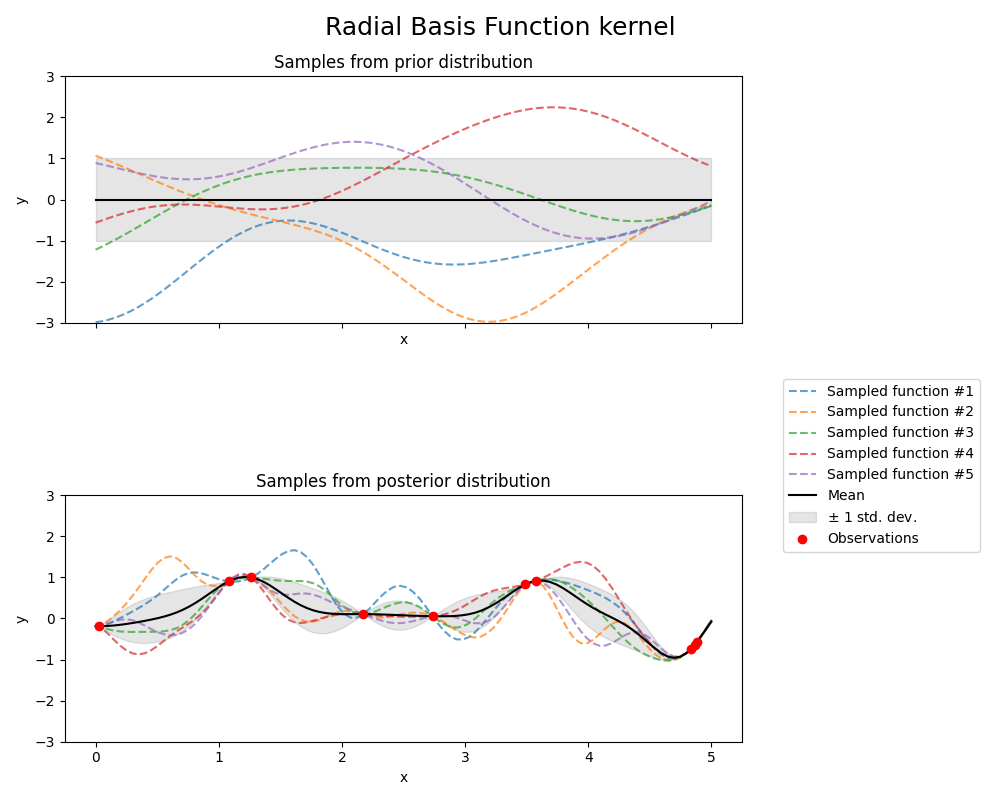
print(f"Kernel parameters before fit:\n{kernel})")
print(
    f"Kernel parameters after fit: \n{gpr.kernel_} \n"
    f"Log-likelihood: {gpr.log_marginal_likelihood(gpr.kernel_.theta):.3f}"
)

Kernel parameters before fit:
1**2 * RBF(length_scale=1))
Kernel parameters after fit:
0.594**2 * RBF(length_scale=0.279)
Log-likelihood: -0.067

有理二次核

from sklearn.gaussian_process.kernels import RationalQuadratic

kernel = 1.0 * RationalQuadratic(length_scale=1.0, alpha=0.1, alpha_bounds=(1e-5, 1e15))
gpr = GaussianProcessRegressor(kernel=kernel, random_state=0)

fig, axs = plt.subplots(nrows=2, sharex=True, sharey=True, figsize=(10, 8))

# plot prior
plot_gpr_samples(gpr, n_samples=n_samples, ax=axs[0])
axs[0].set_title("Samples from prior distribution")

# plot posterior
gpr.fit(X_train, y_train)
plot_gpr_samples(gpr, n_samples=n_samples, ax=axs[1])
axs[1].scatter(X_train[:, 0], y_train, color="red", zorder=10, label="Observations")
axs[1].legend(bbox_to_anchor=(1.05, 1.5), loc="upper left")
axs[1].set_title("Samples from posterior distribution")

fig.suptitle("Rational Quadratic kernel", fontsize=18)
plt.tight_layout()

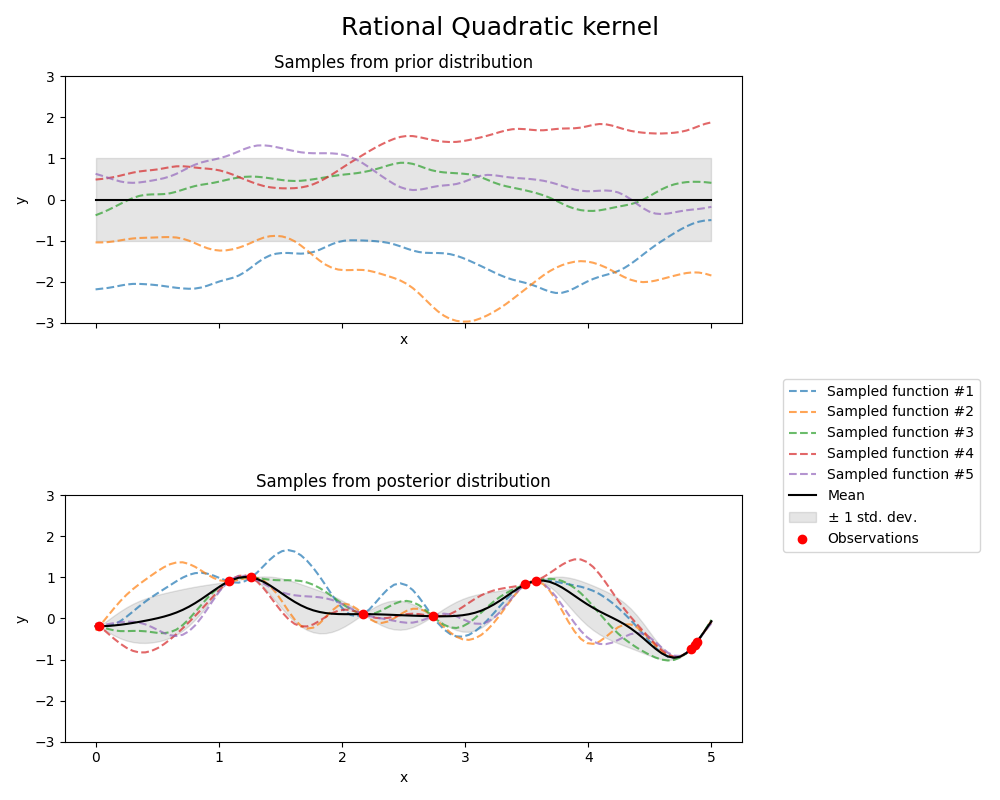
/xpy/lib/python3.11/site-packages/sklearn/gaussian_process/_gpr.py:478: UserWarning:

Predicted variances smaller than 0. Setting those variances to 0.

/xpy/lib/python3.11/site-packages/sklearn/gaussian_process/_gpr.py:523: RuntimeWarning:

covariance is not symmetric positive-semidefinite.

print(f"Kernel parameters before fit:\n{kernel})")
print(
    f"Kernel parameters after fit: \n{gpr.kernel_} \n"
    f"Log-likelihood: {gpr.log_marginal_likelihood(gpr.kernel_.theta):.3f}"
)

Kernel parameters before fit:
1**2 * RationalQuadratic(alpha=0.1, length_scale=1))
Kernel parameters after fit:
0.594**2 * RationalQuadratic(alpha=2.63e+09, length_scale=0.279)
Log-likelihood: -0.064

Exp-Sine-Squared内核

from sklearn.gaussian_process.kernels import ExpSineSquared

kernel = 1.0 * ExpSineSquared(
    length_scale=1.0,
    periodicity=3.0,
    length_scale_bounds=(0.1, 10.0),
    periodicity_bounds=(1.0, 10.0),
)
gpr = GaussianProcessRegressor(kernel=kernel, random_state=0)

fig, axs = plt.subplots(nrows=2, sharex=True, sharey=True, figsize=(10, 8))

# plot prior
plot_gpr_samples(gpr, n_samples=n_samples, ax=axs[0])
axs[0].set_title("Samples from prior distribution")

# plot posterior
gpr.fit(X_train, y_train)
plot_gpr_samples(gpr, n_samples=n_samples, ax=axs[1])
axs[1].scatter(X_train[:, 0], y_train, color="red", zorder=10, label="Observations")
axs[1].legend(bbox_to_anchor=(1.05, 1.5), loc="upper left")
axs[1].set_title("Samples from posterior distribution")

fig.suptitle("Exp-Sine-Squared kernel", fontsize=18)
plt.tight_layout()

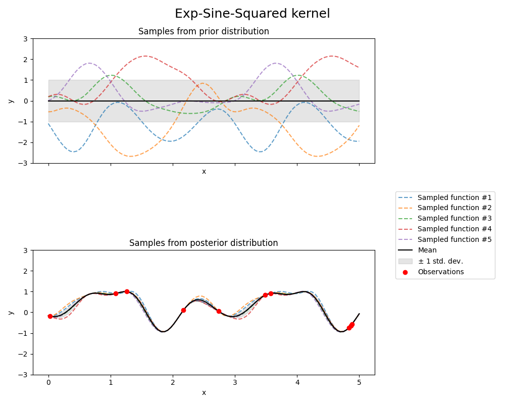
print(f"Kernel parameters before fit:\n{kernel})")
print(
    f"Kernel parameters after fit: \n{gpr.kernel_} \n"
    f"Log-likelihood: {gpr.log_marginal_likelihood(gpr.kernel_.theta):.3f}"
)

Kernel parameters before fit:
1**2 * ExpSineSquared(length_scale=1, periodicity=3))
Kernel parameters after fit:
0.799**2 * ExpSineSquared(length_scale=0.791, periodicity=2.87)
Log-likelihood: 3.394

点积核心

from sklearn.gaussian_process.kernels import ConstantKernel, DotProduct

kernel = ConstantKernel(0.1, (0.01, 10.0)) * (
    DotProduct(sigma_0=1.0, sigma_0_bounds=(0.1, 10.0)) ** 2
)
gpr = GaussianProcessRegressor(kernel=kernel, random_state=0, normalize_y=True)

fig, axs = plt.subplots(nrows=2, sharex=True, sharey=True, figsize=(10, 8))

# plot prior
plot_gpr_samples(gpr, n_samples=n_samples, ax=axs[0])
axs[0].set_title("Samples from prior distribution")

# plot posterior
gpr.fit(X_train, y_train)
plot_gpr_samples(gpr, n_samples=n_samples, ax=axs[1])
axs[1].scatter(X_train[:, 0], y_train, color="red", zorder=10, label="Observations")
axs[1].legend(bbox_to_anchor=(1.05, 1.5), loc="upper left")
axs[1].set_title("Samples from posterior distribution")

fig.suptitle("Dot-product kernel", fontsize=18)
plt.tight_layout()

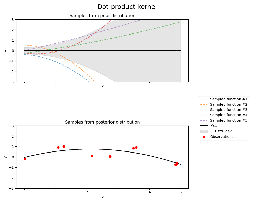
print(f"Kernel parameters before fit:\n{kernel})")
print(
    f"Kernel parameters after fit: \n{gpr.kernel_} \n"
    f"Log-likelihood: {gpr.log_marginal_likelihood(gpr.kernel_.theta):.3f}"
)

Kernel parameters before fit:
0.316**2 * DotProduct(sigma_0=1) ** 2)
Kernel parameters after fit:
0.697**2 * DotProduct(sigma_0=0.454) ** 2
Log-likelihood: -18108182014.707

Matérn核

from sklearn.gaussian_process.kernels import Matern

kernel = 1.0 * Matern(length_scale=1.0, length_scale_bounds=(1e-1, 10.0), nu=1.5)
gpr = GaussianProcessRegressor(kernel=kernel, random_state=0)

fig, axs = plt.subplots(nrows=2, sharex=True, sharey=True, figsize=(10, 8))

# plot prior
plot_gpr_samples(gpr, n_samples=n_samples, ax=axs[0])
axs[0].set_title("Samples from prior distribution")

# plot posterior
gpr.fit(X_train, y_train)
plot_gpr_samples(gpr, n_samples=n_samples, ax=axs[1])
axs[1].scatter(X_train[:, 0], y_train, color="red", zorder=10, label="Observations")
axs[1].legend(bbox_to_anchor=(1.05, 1.5), loc="upper left")
axs[1].set_title("Samples from posterior distribution")

fig.suptitle("Matérn kernel", fontsize=18)
plt.tight_layout()

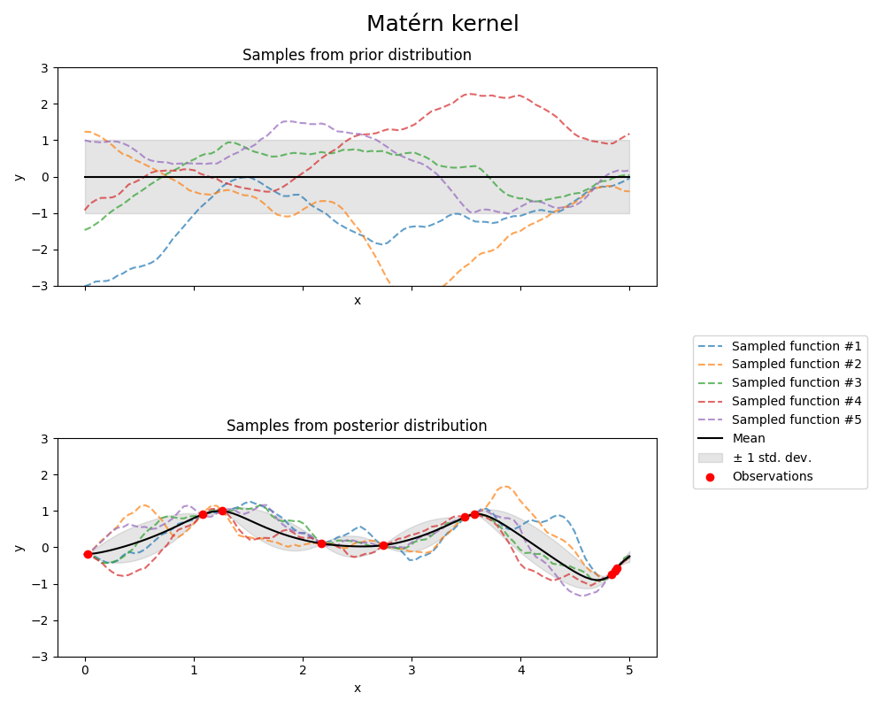
print(f"Kernel parameters before fit:\n{kernel})")
print(
    f"Kernel parameters after fit: \n{gpr.kernel_} \n"
    f"Log-likelihood: {gpr.log_marginal_likelihood(gpr.kernel_.theta):.3f}"
)

Kernel parameters before fit:
1**2 * Matern(length_scale=1, nu=1.5))
Kernel parameters after fit:
0.609**2 * Matern(length_scale=0.484, nu=1.5)
Log-likelihood: -1.185

相关实例

高斯过程回归（GPT）估计数据噪音水平的能力

Ability of Gaussian process regression (GPR) to estimate data noise-level

k均值假设的证明

Demonstration of k-means assumptions

二分K均值和常规K均值性能比较

Bisecting K-Means and Regular K-Means Performance Comparison

高斯过程回归：基本入门示例

Gaussian Processes regression: basic introductory example