1.7. 高斯过程#
Gaussian Processes (GP) 是一种非参数监督学习方法,用于解决 regression 和 probabilistic classification 问题
高斯过程的优点是:
预测对观察结果进行内插(至少对于常规核)。
预测是概率的(高斯),以便可以计算经验置信区间,并根据这些置信区间决定是否应该重新调整(在线匹配、自适应匹配)某个感兴趣区域的预测。
多才多艺:不同 kernels 可以指定。提供了通用内核,但也可以指定自定义内核。
高斯过程的缺点包括:
我们的实现并不稀疏,即他们使用整个样本/特征信息来执行预测。
它们在多维空间中失去效率--即当特征数量超过几十个时。
1.7.1. 高斯过程回归(GPT)#
的 GaussianProcessRegressor 出于回归目的实现高斯过程(GP)。为此,需要指定GP的前任。GP将根据训练样本将此先验信息和似然函数结合起来。它允许通过在预测时给出均值和标准差作为输出来给出概率预测方法。
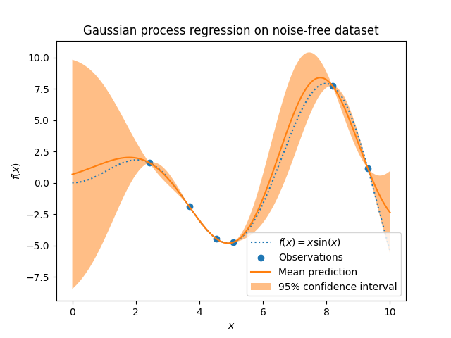
假设先验均值为常数和零(对于 normalize_y=False )或训练数据的平均值(对于 normalize_y=True ).先验的协方差通过传递指定 kernel object.在匹配时优化了内核的超参数 GaussianProcessRegressor 通过最大化对数边际似然(LML), optimizer .由于LML可能有多个本地优化,因此可以通过指定来重复启动优化器 n_restarts_optimizer .第一次运行始终从内核的初始超参数值开始进行;后续运行是从允许值范围中随机选择的超参数值进行的。如果初始超参数应该保持固定, None 可以作为优化器传递。
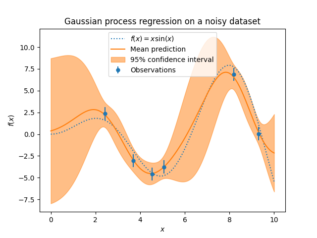
目标中的噪音水平可以通过参数传递来指定 alpha 全局标量或每个数据点。请注意,适度的噪音水平也有助于处理匹配期间的数字不稳定性,因为它有效地实现为Tikhonov正规化,即通过将其添加到核矩阵的对角线上。显式指定噪声水平的替代方案是包括 WhiteKernel 将组件添加到内核中,该内核可以根据数据估计全局噪音水平(请参阅下面的示例)。下图显示了通过设置参数处理的有噪目标的影响 alpha .
该实现基于的算法2.1 [RW2006]. 除了标准scikit-learn估计器的API之外, GaussianProcessRegressor :
允许在没有先验匹配的情况下进行预测(基于GP先验)
提供了额外的方法
sample_y(X),它评估在给定输入下从GPT(之前或之后)提取的样本暴露一种方法
log_marginal_likelihood(theta),它可以在外部用于选择超参数的其他方式,例如,通过马尔科夫链蒙特卡洛。
示例
1.7.2. 高斯过程分类(GSK)#
的 GaussianProcessClassifier 实现高斯过程(GP)用于分类目的,更具体地用于概率分类,其中测试预测采用类别概率的形式。GaussianProcess Classifier将GP置于潜在函数之上 \(f\) ,然后通过链接函数将其压缩 \(\pi\) 以获得概率分类。潜在功能 \(f\) 是一个所谓的滋扰函数,其值不被观察,并且本身不相关。其目的是方便地制定模型,并且 \(f\) 在预测期间被删除(积分)。 GaussianProcessClassifier 实现了逻辑链路函数,其积分无法解析计算,但在二进制情况下很容易近似。
与回归设置相反,潜函数的后验 \(f\) 即使对于GP先验也不是高斯的,因为高斯似然不适合离散类别标签。相反,使用与逻辑链接函数(logit)相对应的非高斯似然。GaussianProcess Classifier基于拉普拉斯逼近用高斯逼近非高斯后验。更多详细信息请参阅的第3章 [RW2006].
假设GP先验平均值为零。先验的协方差通过传递指定 kernel object.在GaussianProcessRegressor的拟合过程中,通过基于传递函数的最大化对数边际似然(LML)来优化核的超参数。 optimizer .由于LML可能有多个本地优化,因此可以通过指定来重复启动优化器 n_restarts_optimizer .第一次运行始终从内核的初始超参数值开始进行;后续运行是从允许值范围中随机选择的超参数值进行的。如果初始超参数应该保持固定, None 可以作为优化器传递。
在某些情况下,关于潜在功能的信息 \(f\) 是期望的(即平均值 \(\bar{f_*}\) 和方差 \(\text{Var}[f_*]\) 在方程中描述。(3.21)和(3.24)的 [RW2006]) .的 GaussianProcessClassifier 通过 latent_mean_and_variance 法
GaussianProcessClassifier 通过执行基于一对一或基于一对一的训练和预测来支持多类分类。 在one-versus-rest中,为每个类拟合一个二进制高斯过程分类器,该分类器经过训练以将该类与其余类分开。在“one_vs_one”中,为每对类安装一个二进制高斯过程分类器,并训练该分类器以分离这两个类。这些二元预测器的预测被组合成多类预测。参阅中的一节 multi-class classification 了解更多详细信息。
在高斯过程分类的情况下,“one_vs_one”可能在计算上更便宜,因为它必须解决仅涉及整个训练集的一个子集的许多问题,而不是整个数据集中的更少问题。由于高斯过程分类随着数据集的大小而按立方比例缩放,因此这可能会快得多。然而,请注意,“one_vs_one”不支持预测概率估计,而仅支持简单的预测。此外,请注意, GaussianProcessClassifier (尚未)在内部实现真正的多类拉普拉斯逼近,但如上所述,它基于在内部解决几个二元分类任务,这些任务使用一对一或一对一进行组合。
1.7.3. 凝胶渗透控制示例#
1.7.3.1. 使用PCR进行概率预测#
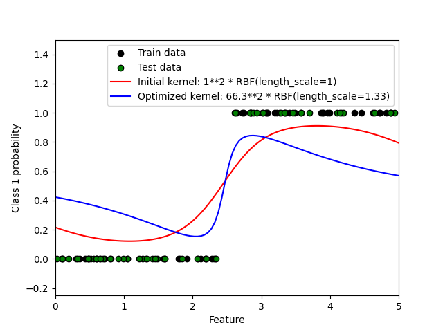
此示例说明了具有不同超参数选择的RBS核的预测概率。第一个图显示了具有任意选择的超参数以及与最大log边际似然(LML)相对应的超参数的预测概率。
虽然通过优化LML选择的超参数具有相当大的LML,但根据测试数据的对数损失,它们的性能稍差。该图显示,这是因为它们在类边界处表现出类概率的急剧变化(这很好),但在远离类边界的地方预测概率接近0.5(这很糟糕)。这种不良影响是由GSK内部使用的拉普拉斯逼近引起的。
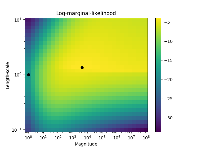
第二个图显示了内核超参数不同选择的log边际似然,并用黑点突出显示了第一个图中使用的超参数的两种选择。
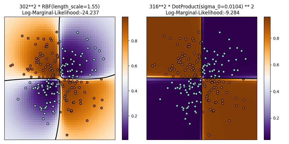
1.7.3.2. 异或数据集上的PCR插图#
此示例说明了异或数据上的CPC。相比之下是一个稳定的、各向同性的核 (RBF )和非静态内核 (DotProduct ).在这个特定的数据集上, DotProduct 核获得了更好的结果,因为类边界是线性的并且与坐标轴重合。然而,在实践中,固定内核,例如 RBF 往往会获得更好的结果。
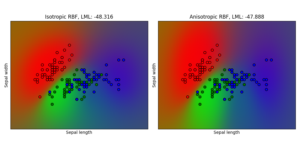
1.7.3.3. 虹膜数据集上的高斯过程分类(GSK)#
此示例说明了虹膜数据集的二维版本上各向同性和各向异性的RBS核的预测概率。这说明了CPC对非二元分类的适用性。通过为两个特征维度分配不同的长度尺度,各向异性的RBS核获得稍高的log边际似然度。
1.7.4. 高斯过程的核#
核(在GP的上下文中也称为“协方差函数”)是GP的关键组成部分,它决定GP的前和后形状。它们通过定义两个数据点的“相似性”并结合相似数据点应该具有相似目标值的假设,对所学习的函数的假设进行编码。可以区分两类核:静止核仅取决于两个数据点的距离,而不取决于它们的绝对值 \(k(x_i, x_j)= k(d(x_i, x_j))\) 因此,对于输入空间中的翻译是不变的,而非平稳核也取决于数据点的特定值。静止核可以进一步细分为各向同性核和各向异性核,其中各向同性核也不受输入空间中的旋转的影响。有关更多详细信息,请参阅的第4章 [RW2006]. This example 展示如何在离散数据上定义自定义内核。有关如何最好地组合不同内核的指导,请参阅 [Duv2014].
高斯过程核心API#
a的主要用途 Kernel 是计算GP数据点之间的协方差。为此,方法 __call__ 可以调用内核的。该方法可以用于计算2d阵列X中所有数据点对的“自协方差”,也可以用于计算2d阵列X的数据点与2d阵列Y中数据点的所有组合的“交叉协方差”。以下身份对于所有内核k都成立(除了 WhiteKernel ): k(X) == K(X, Y=X)
如果仅使用自协方差的对角线,则该方法 diag() 可以调用内核的,这比对 __call__ : np.diag(k(X, X)) == k.diag(X)
Kernels are parameterized by a vector \(\theta\) of hyperparameters. These
hyperparameters can for instance control length-scales or periodicity of a
kernel (see below). All kernels support computing analytic gradients
of the kernel's auto-covariance with respect to \(log(\theta)\) via setting
eval_gradient=True in the __call__ method.
That is, a (len(X), len(X), len(theta)) array is returned where the entry
[i, j, l] contains \(\frac{\partial k_\theta(x_i, x_j)}{\partial log(\theta_l)}\).
This gradient is used by the Gaussian process (both regressor and classifier)
in computing the gradient of the log-marginal-likelihood, which in turn is used
to determine the value of \(\theta\), which maximizes the log-marginal-likelihood,
via gradient ascent. For each hyperparameter, the initial value and the
bounds need to be specified when creating an instance of the kernel. The
current value of \(\theta\) can be get and set via the property
theta of the kernel object. Moreover, the bounds of the hyperparameters can be
accessed by the property bounds of the kernel. Note that both properties
(theta and bounds) return log-transformed values of the internally used values
since those are typically more amenable to gradient-based optimization.
The specification of each hyperparameter is stored in the form of an instance of
Hyperparameter in the respective kernel. Note that a kernel using a
hyperparameter with name "x" must have the attributes self.x and self.x_bounds.
所有内核的抽象基本类是 Kernel .内核实现了类似的接口 BaseEstimator ,提供方法 get_params() , set_params() ,而且 clone() .这还允许通过元估计器设置内核值,例如 Pipeline 或 GridSearchCV .注意,由于内核的嵌套结构(通过应用内核运算符,见下文),内核参数的名称可能会变得相对复杂。通常,对于二元核运算符,左操作数的参数以 k1__ 和右操作数的参数 k2__ .另一种方便的方法是 clone_with_theta(theta) ,它返回内核的克隆版本,但超参数设置为 theta .一个说明性的例子:
>>> from sklearn.gaussian_process.kernels import ConstantKernel, RBF
>>> kernel = ConstantKernel(constant_value=1.0, constant_value_bounds=(0.0, 10.0)) * RBF(length_scale=0.5, length_scale_bounds=(0.0, 10.0)) + RBF(length_scale=2.0, length_scale_bounds=(0.0, 10.0))
>>> for hyperparameter in kernel.hyperparameters: print(hyperparameter)
Hyperparameter(name='k1__k1__constant_value', value_type='numeric', bounds=array([[ 0., 10.]]), n_elements=1, fixed=False)
Hyperparameter(name='k1__k2__length_scale', value_type='numeric', bounds=array([[ 0., 10.]]), n_elements=1, fixed=False)
Hyperparameter(name='k2__length_scale', value_type='numeric', bounds=array([[ 0., 10.]]), n_elements=1, fixed=False)
>>> params = kernel.get_params()
>>> for key in sorted(params): print("%s : %s" % (key, params[key]))
k1 : 1**2 * RBF(length_scale=0.5)
k1__k1 : 1**2
k1__k1__constant_value : 1.0
k1__k1__constant_value_bounds : (0.0, 10.0)
k1__k2 : RBF(length_scale=0.5)
k1__k2__length_scale : 0.5
k1__k2__length_scale_bounds : (0.0, 10.0)
k2 : RBF(length_scale=2)
k2__length_scale : 2.0
k2__length_scale_bounds : (0.0, 10.0)
>>> print(kernel.theta)  # Note: log-transformed
[ 0.         -0.69314718  0.69314718]
>>> print(kernel.bounds)  # Note: log-transformed
[[      -inf 2.30258509]
[      -inf 2.30258509]
[      -inf 2.30258509]]
所有高斯过程内核都可与 sklearn.metrics.pairwise 反之亦然:子类的实例 Kernel 可以通过作为 metric 到 pairwise_kernels 从 sklearn.metrics.pairwise .此外,通过使用包装器类,成对的内核函数可以用作GP内核 PairwiseKernel .唯一需要注意的是,超参数的梯度不是解析的,而是数值的,并且所有这些内核都只支持各向同性距离。参数 gamma 被认为是超参数并且可以被优化。其他内核参数在初始化时直接设置,并保持固定。
1.7.4.1. 基本内核#
的 ConstantKernel 内核可以用作 Product 内核,其中它缩放其他因素(内核)的大小或作为 Sum 内核,其中它修改高斯过程的平均值。这取决于参数 \(constant\_value\) .它的定义是:
的主要用例 WhiteKernel 内核是总和内核的一部分,它解释信号的噪音分量。调整其参数 \(noise\_level\) 对应于估计噪音水平。它的定义是:
1.7.4.2. 核运算符#
Kernel operators take one or two base kernels and combine them into a new
kernel. The Sum kernel takes two kernels \(k_1\) and \(k_2\)
and combines them via \(k_{sum}(X, Y) = k_1(X, Y) + k_2(X, Y)\).
The Product kernel takes two kernels \(k_1\) and \(k_2\)
and combines them via \(k_{product}(X, Y) = k_1(X, Y) * k_2(X, Y)\).
The Exponentiation kernel takes one base kernel and a scalar parameter
\(p\) and combines them via
\(k_{exp}(X, Y) = k(X, Y)^p\).
Note that magic methods __add__, __mul___ and __pow__ are
overridden on the Kernel objects, so one can use e.g. RBF() + RBF() as
a shortcut for Sum(RBF(), RBF()).
1.7.4.3. 辐射基函数(RBS)核#
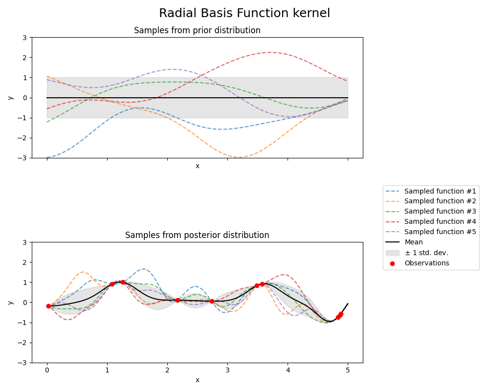
的 RBF 内核是一个固定的内核。它也被称为“平方指数”核。它由长度比例参数参数化 \(l>0\) ,它可以是一个纯量(内核的各向同性变体),也可以是与输入具有相同维度的载体 \(x\) (内核的各向异性变体)。内核由下式给出:
哪里 \(d(\cdot, \cdot)\) 是欧几里得距离。该核是无限可微的,这意味着以该核作为协方差函数的GP具有所有阶的均方求导,因此非常光滑。下图显示了由RBS核产生的GP的先验和后验:
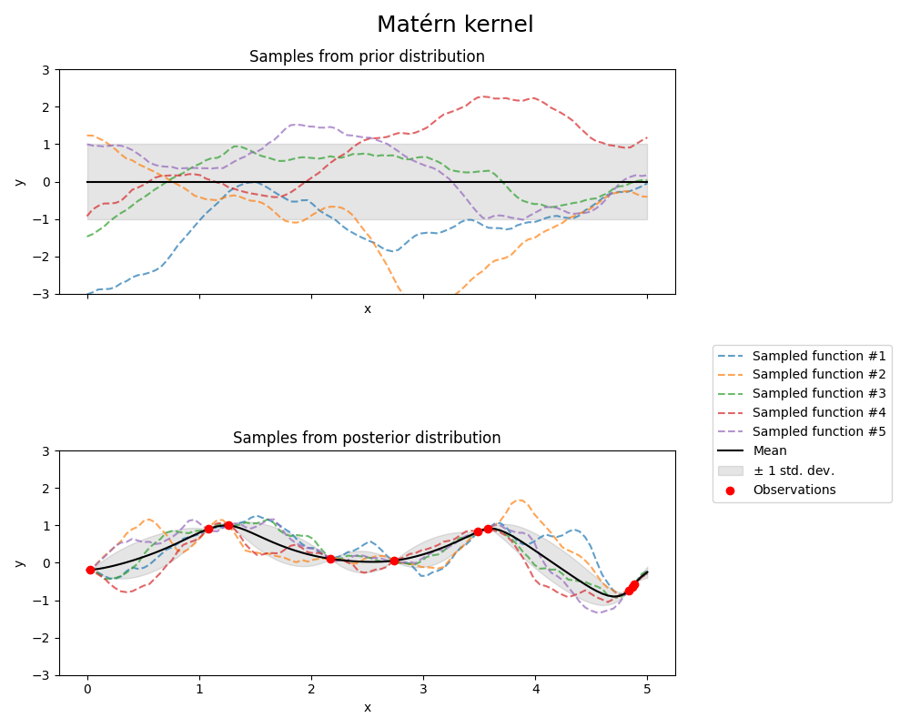
1.7.4.4. Matérn核#
的 Matern 核是一个平稳的核和推广的 RBF 内核。它有一个额外的参数 \(\nu\) 它控制生成函数的平滑度。它由长度比例参数参数化 \(l>0\) ,它可以是一个纯量(内核的各向同性变体),也可以是与输入具有相同维度的载体 \(x\) (内核的各向异性变体)。
Matérn内核的数学实现#
内核由下式给出:
where \(d(\cdot,\cdot)\) is the Euclidean distance, \(K_\nu(\cdot)\) is a modified Bessel function and \(\Gamma(\cdot)\) is the gamma function. As \(\nu\rightarrow\infty\), the Matérn kernel converges to the RBF kernel. When \(\nu = 1/2\), the Matérn kernel becomes identical to the absolute exponential kernel, i.e.,
特别是, \(\nu = 3/2\) :
和 \(\nu = 5/2\) :
对于不是无限可微(如RBS核所假设的)但至少可微一次的学习函数来说,是流行的选择 (\(\nu = 3/2\) )或两次可微 (\(\nu = 5/2\) ).
控制学习函数平滑度的灵活性, \(\nu\) 允许适应真正的基础功能关系的属性。
下图显示了由Matérn内核产生的GP的先验和后验:
看到 [RW2006], 第84页,了解有关Matérn内核不同变体的更多详细信息。
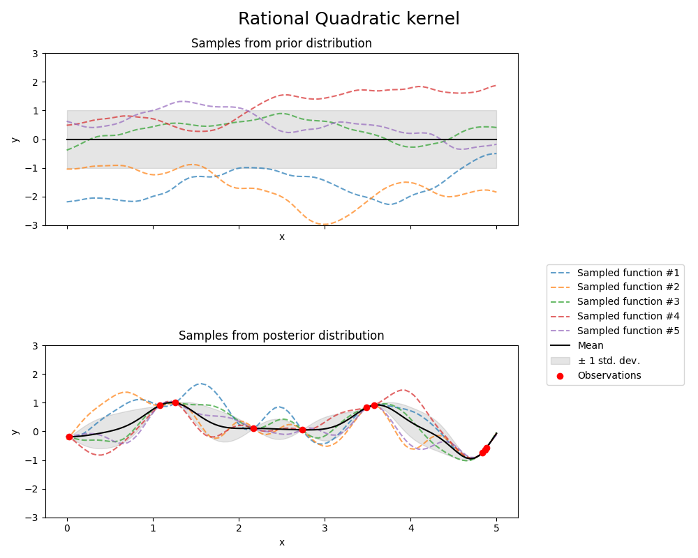
1.7.4.5. 有理二次核#
的 RationalQuadratic 内核可以被视为以下的规模混合物(无限和) RBF 具有不同特征长度尺度的籽粒。它由长度比例参数参数化 \(l>0\) 和规模混合参数 \(\alpha>0\) 只有各向同性变体, \(l\) 是目前支持的纯量。内核由下式给出:
全科医生的先验和先验 RationalQuadratic 内核如下图所示:
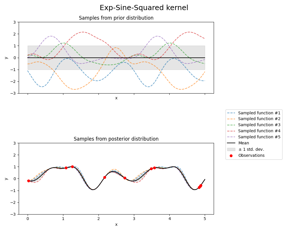
1.7.4.6. Exp-Sine-Squared内核#
的 ExpSineSquared 内核允许对周期性函数进行建模。它由长度比例参数参数化 \(l>0\) 和周期性参数 \(p>0\) .只有各向同性变体, \(l\) 是目前支持的纯量。内核由下式给出:
The prior and posterior of a GP resulting from an ExpSineSquared kernel are shown in the following figure:
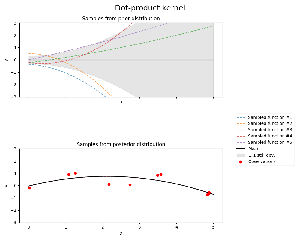
1.7.4.7. 点积内核#
The DotProduct kernel is non-stationary and can be obtained from linear regression
by putting \(N(0, 1)\) priors on the coefficients of \(x_d (d = 1, . . . , D)\) and
a prior of \(N(0, \sigma_0^2)\) on the bias. The DotProduct kernel is invariant to a rotation
of the coordinates about the origin, but not translations.
It is parameterized by a parameter \(\sigma_0^2\). For \(\sigma_0^2 = 0\), the kernel
is called the homogeneous linear kernel, otherwise it is inhomogeneous. The kernel is given by
的 DotProduct 内核通常与取指数相结合。下图显示了指数为2的示例:
1.7.4.8. 引用#
Carl E. Rasmussen and Christopher K.I. Williams, "Gaussian Processes for Machine Learning", MIT Press 2006 <https://www.gaussianprocess.org/gpml/chapters/RW.pdf> _
David Duvenaud, "The Kernel Cookbook: Advice on Covariance functions", 2014 <https://www.cs.toronto.edu/~duvenaud/cookbook/> _