1.17. 神经网络模型(监督)#
警告
此实现不适用于大规模应用程序。特别是,scikit-learn不提供图形处理器支持。如需更快的基于GOP的实施,以及为构建深度学习架构提供更大灵活性的框架,请参阅 相关项目 .
1.17.1. 多层感知器#
Multi-layer Perceptron (MLP) is a supervised learning algorithm that learns a function \(f: R^m \rightarrow R^o\) by training on a dataset, where \(m\) is the number of dimensions for input and \(o\) is the number of dimensions for output. Given a set of features \(X = {x_1, x_2, ..., x_m}\) and a target \(y\), it can learn a non-linear function approximator for either classification or regression. It is different from logistic regression, in that between the input and the output layer, there can be one or more non-linear layers, called hidden layers. Figure 1 shows a one hidden layer MLP with scalar output.
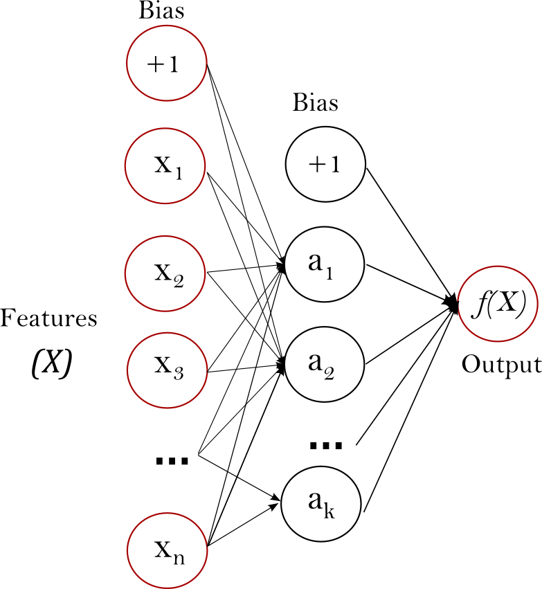
Figure 1 : One hidden layer MLP.#
The leftmost layer, known as the input layer, consists of a set of neurons \(\{x_i | x_1, x_2, ..., x_m\}\) representing the input features. Each neuron in the hidden layer transforms the values from the previous layer with a weighted linear summation \(w_1x_1 + w_2x_2 + ... + w_mx_m\), followed by a non-linear activation function \(g(\cdot):R \rightarrow R\) - like the hyperbolic tan function. The output layer receives the values from the last hidden layer and transforms them into output values.
模块包含公共属性 coefs_ 和 intercepts_ . coefs_ 是权重矩阵列表,其中权重矩阵位于索引处 \(i\) 代表层之间的权重 \(i\) 和层 \(i+1\) . intercepts_ 是偏置载体列表,其中索引处的载体 \(i\) 代表添加到层的偏差值 \(i+1\) .
多层感知器的优点和缺点#
多层感知器的优点是:
学习非线性模型的能力。
能够使用实时学习模型(在线学习)
partial_fit.
The disadvantages of Multi-layer Perceptron (MLP) include:
具有隐藏层的MLP具有非凸损失函数,其中存在多个局部最小值。因此,不同的随机权重初始化可以导致不同的验证精度。
MLP需要调整许多超参数,例如隐藏神经元、层和迭代的数量。
MLP对特征缩放很敏感。
请参阅 Tips on Practical Use 解决其中一些缺点的部分。
1.17.2. 分类#
类 MLPClassifier 实现多层感知器(MLP)算法,该算法使用 Backpropagation .
MLP在两个阵列上训练:大小为(n_samples,n_features)的数组X,保存表示为浮点特征载体的训练样本;大小为(n_samples,)的数组y,保存训练样本的目标值(类标签)::
>>> from sklearn.neural_network import MLPClassifier
>>> X = [[0., 0.], [1., 1.]]
>>> y = [0, 1]
>>> clf = MLPClassifier(solver='lbfgs', alpha=1e-5,
...                     hidden_layer_sizes=(5, 2), random_state=1)
...
>>> clf.fit(X, y)
MLPClassifier(alpha=1e-05, hidden_layer_sizes=(5, 2), random_state=1,
              solver='lbfgs')
拟合(训练)后,模型可以预测新样本的标签:
>>> clf.predict([[2., 2.], [-1., -2.]])
array([1, 0])
MLP可以将非线性模型与训练数据进行匹配。 clf.coefs_ 包含构成模型参数的权重矩阵::
>>> [coef.shape for coef in clf.coefs_]
[(2, 5), (5, 2), (2, 1)]
目前, MLPClassifier 仅支持交叉熵损失函数,该函数允许通过运行 predict_proba 法
MLP使用反向传播进行训练。更准确地说,它使用某种形式的梯度下降进行训练,并使用反向传播计算梯度。对于分类,它最小化了交叉熵损失函数,从而给出了概率估计的载体 \(P(y|x)\) 每个样品 \(x\)
>>> clf.predict_proba([[2., 2.], [1., 2.]])
array([[1.967e-04, 9.998e-01],
       [1.967e-04, 9.998e-01]])
MLPClassifier 应用支持多类别分类 Softmax 作为输出函数。
Further, the model supports multi-label classification
in which a sample can belong to more than one class. For each class, the raw
output passes through the logistic function. Values larger or equal to 0.5
are rounded to 1, otherwise to 0. For a predicted output of a sample, the
indices where the value is 1 represent the assigned classes of that sample:
>>> X = [[0., 0.], [1., 1.]]
>>> y = [[0, 1], [1, 1]]
>>> clf = MLPClassifier(solver='lbfgs', alpha=1e-5,
...                     hidden_layer_sizes=(15,), random_state=1)
...
>>> clf.fit(X, y)
MLPClassifier(alpha=1e-05, hidden_layer_sizes=(15,), random_state=1,
              solver='lbfgs')
>>> clf.predict([[1., 2.]])
array([[1, 1]])
>>> clf.predict([[0., 0.]])
array([[0, 1]])
请参阅下面的示例和 MLPClassifier.fit 获取更多信息.
示例
看到 MNIST上MLP权重的可视化 用于训练权重的可视化表示。
1.17.3. 回归#
类 MLPRegressor 实现多层感知器(MLP),其使用反向传播进行训练,输出层中没有激活函数,这也可以被视为使用身份函数作为激活函数。因此,它使用平方误差作为损失函数,输出是一组连续的值。
MLPRegressor 还支持多输出回归,其中一个样本可以有多个目标。
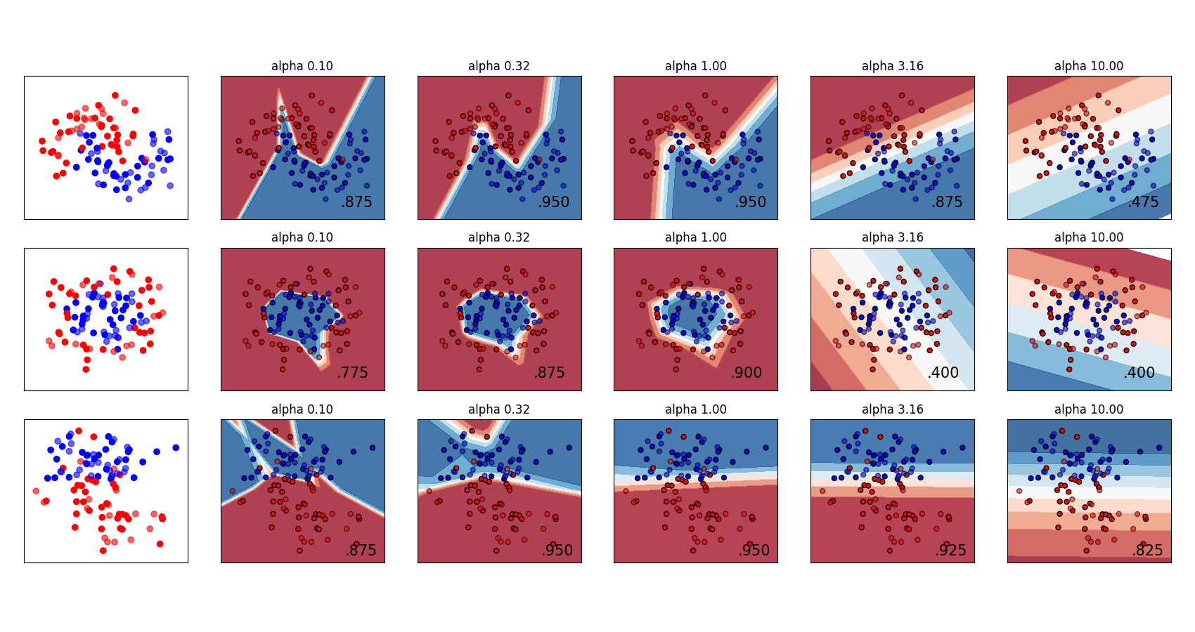
1.17.4. 正则化#
两 MLPRegressor 和 MLPClassifier 使用参数 alpha 对于正则化(L2正则化)项,这有助于通过惩罚具有大幅度的权重来避免过拟合。下图显示了具有alpha值的不同决策函数。
有关更多信息,请参阅下面的示例。
示例
1.17.5. 算法#
MLP列车使用 Stochastic Gradient Descent, Adam, or L-BFGS .随机梯度下降(SDP)使用损失函数相对于需要自适应的参数(即
哪里 \(\eta\) 是控制参数空间搜索中步进大小的学习率。 \(Loss\) 是用于网络的损失函数。
更多详细信息请参阅 SGD
Adam在某种意义上类似于Singapore,它是一个随机优化器,但它可以根据较低阶矩的自适应估计自动调整更新参数的量。
通过Singapore或Adam,培训支持在线和小批量学习。
L-BFGS是一个近似Hessian矩阵的求解器,Hessian矩阵表示函数的二阶偏导数。进一步地,它近似Hessian矩阵的逆以执行参数更新。该实现使用Scipy版本的 L-BFGS .
如果选择的求解器是“L-BFSG”,则训练不支持在线或小批量学习。
1.17.6. 复杂性#
Suppose there are \(n\) training samples, \(m\) features, \(k\) hidden layers, each containing \(h\) neurons - for simplicity, and \(o\) output neurons. The time complexity of backpropagation is \(O(i \cdot n \cdot (m \cdot h + (k - 1) \cdot h \cdot h + h \cdot o))\), where \(i\) is the number of iterations. Since backpropagation has a high time complexity, it is advisable to start with smaller number of hidden neurons and few hidden layers for training.
数学公式#
Given a set of training examples \((x_1, y_1), (x_2, y_2), \ldots, (x_n, y_n)\) where \(x_i \in \mathbf{R}^n\) and \(y_i \in \{0, 1\}\), a one hidden layer one hidden neuron MLP learns the function \(f(x) = W_2 g(W_1^T x + b_1) + b_2\) where \(W_1 \in \mathbf{R}^m\) and \(W_2, b_1, b_2 \in \mathbf{R}\) are model parameters. \(W_1, W_2\) represent the weights of the input layer and hidden layer, respectively; and \(b_1, b_2\) represent the bias added to the hidden layer and the output layer, respectively. \(g(\cdot) : R \rightarrow R\) is the activation function, set by default as the hyperbolic tan. It is given as,
对于二元分类, \(f(x)\) 经过后勤职能 \(g(z)=1/(1+e^{-z})\) 以获得0和1之间的输出值。设置为0.5的阈值将把大于或等于0.5的输出样本分配给正类,其余的分配给负类。
如果有两个以上的班级, \(f(x)\) 其本身将是一个大小(n_classes,)的载体。它不是通过逻辑函数,而是通过softmax函数,该函数被写为,
哪里 \(z_i\) 代表 \(i\) softmax输入的第th个元素,对应于类 \(i\) ,而且 \(K\) 是类的数量。结果是一个包含抽样概率的载体 \(x\) 属于每个班级。输出是概率最高的类。
在回归中,输出仍然是 \(f(x)\) 因此,输出激活函数就是恒等函数。
MLP根据问题类型使用不同的损失函数。分类的损失函数是平均交叉熵,在二进制情况下给出为,
哪里 \(\alpha ||W||_2^2\) 是一个L2正规化项(又名罚分),用于惩罚复杂模型;并且 \(\alpha > 0\) 是控制处罚幅度的非负超参数。
对于回归,MLP使用均方误差损失函数;写成,
多层感知器(MLP)从初始随机权重开始,通过重复更新这些权重来最小化损失函数。计算损失后,向后传递将其从输出层传播到之前的层,为每个权重参数提供旨在减少损失的更新值。
在梯度下降中,梯度 \(\nabla Loss_{W}\) 计算并从以下公式中扣除相对于权重的损失 \(W\) .更正式地说,这被表达为,
哪里 \(i\) 是迭代步骤,并且 \(\epsilon\) 是值大于0的学习率。
当达到预设的最大迭代次数时,算法就会停止;或者当损失的改善低于某个较小的数字时。
1.17.7. 实际使用技巧#
多层Perceptron对特征扩展很敏感,因此强烈建议扩展您的数据。例如,将输入载体X上的每个属性缩放为 [0, 1] 或 [-1, +1] ,或将其标准化以使其均值为0和方差为1。请注意,您必须应用 same 扩展到测试集以获得有意义的结果。您可以使用
StandardScaler为了标准化。>>> from sklearn.preprocessing import StandardScaler >>> scaler = StandardScaler() >>> # Don't cheat - fit only on training data >>> scaler.fit(X_train) >>> X_train = scaler.transform(X_train) >>> # apply same transformation to test data >>> X_test = scaler.transform(X_test)
另一种推荐的方法是使用
StandardScaler中Pipeline寻找合理的正规化参数 \(\alpha\) 最好使用
GridSearchCV,通常在范围内10.0 ** -np.arange(1, 7).根据经验,我们观察到
L-BFGS更快地收敛,并在小型数据集上提供更好的解决方案。然而,对于相对较大的数据集,Adam非常强大。它通常收敛得很快,并提供相当好的性能。SGD另一方面,如果学习率得到正确调整,具有动量或nesterov动量的算法可以比这两种算法表现得更好。
1.17.8. 使用warm_start提供更多控制#
如果您希望对停止标准或新加坡元学习率进行更多控制,或者想要进行额外监控,请使用 warm_start=True 和 max_iter=1 并迭代自己可能会有所帮助::
>>> X = [[0., 0.], [1., 1.]]
>>> y = [0, 1]
>>> clf = MLPClassifier(hidden_layer_sizes=(15,), random_state=1, max_iter=1, warm_start=True)
>>> for i in range(10):
...     clf.fit(X, y)
...     # additional monitoring / inspection
MLPClassifier(...
引用#
"Learning representations by back-propagating errors." 鲁梅尔哈特,大卫·E.,杰弗里·E辛顿和罗纳德·J·威廉姆斯。
"Stochastic Gradient Descent" L. Bottou -网站,2010年。
"Backpropagation" Andrew Ng,Jiquan Ngiam,Chuan Yu Foo,Yifan Mai,Caroline Suen - Website,2011.
"Efficient BackProp" Y.莱昆湖博图,G.奥尔,K.穆勒-《神经网络:贸易技巧》1998年。
"Adam: A method for stochastic optimization." Kingma、Diederik和Jimmy Ba(2014)