6. 可视化#
Scikit-learn定义了一个简单的API,用于创建机器学习的可视化。此API的关键功能是允许快速绘制和视觉调整,而无需重新计算。我们提供 Display 公开两种创建图的方法的类: from_estimator 和 from_predictions .
的 from_estimator 方法生成 Display 来自匹配估计器的对象、输入数据 (X , y ),还有情节。的 from_predictions 方法创建一个 Display 从真实值和预测值中提取对象 (y_test , y_pred ),还有情节。
Using from_predictions avoids having to recompute predictions,
but the user needs to take care that the prediction values passed correspond
to the pos_label. For predict_proba, select the column corresponding
to the pos_label class while for decision_function, revert the score
(i.e. multiply by -1) if pos_label is not the last class in the
classes_ attribute of your estimator.
的 Display 对象存储计算出的值(例如,指标值或特征重要性)使用Matplotlib绘制所需的。这些值是从传递给 from_predictions ,或估计器, X 传递给 from_estimator .
显示对象具有一个plot方法,一旦显示对象初始化,该方法就会创建matplotlib plot(请注意,我们建议通过 from_estimator 或 from_predictions 而不是直接初始化)。地块方法允许通过传递现有地块添加到现有地块 matplotlib.axes.Axes 到 ax 参数.
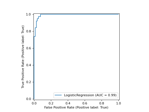
在下面的示例中,我们绘制了适合的逻辑回归模型的ROC曲线 from_estimator :
from sklearn.model_selection import train_test_split
from sklearn.linear_model import LogisticRegression
from sklearn.metrics import RocCurveDisplay
from sklearn.datasets import load_iris

X, y = load_iris(return_X_y=True)
y = y == 2  # make binary
X_train, X_test, y_train, y_test = train_test_split(
   X, y, test_size=.8, random_state=42
)
clf = LogisticRegression(random_state=42, C=.01)
clf.fit(X_train, y_train)

clf_disp = RocCurveDisplay.from_estimator(clf, X_test, y_test)
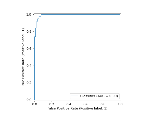
如果您已经拥有预测值,则可以使用 from_predictions 要做同样的事情(并保存在计算机上):
from sklearn.model_selection import train_test_split
from sklearn.linear_model import LogisticRegression
from sklearn.metrics import RocCurveDisplay
from sklearn.datasets import load_iris

X, y = load_iris(return_X_y=True)
y = y == 2  # make binary
X_train, X_test, y_train, y_test = train_test_split(
   X, y, test_size=.8, random_state=42
)
clf = LogisticRegression(random_state=42, C=.01)
clf.fit(X_train, y_train)

# select the probability of the class that we considered to be the positive label
y_pred = clf.predict_proba(X_test)[:, 1]

clf_disp = RocCurveDisplay.from_predictions(y_test, y_pred)
返回的 clf_disp 对象允许我们将另一条曲线添加到已经计算的ROC曲线。本案中 clf_disp 是一 RocCurveDisplay 它将计算值存储为称为 roc_auc , fpr ,而且 tpr .
接下来,我们训练随机森林分类器,并使用 plot 方法 Display object.
import matplotlib.pyplot as plt
from sklearn.ensemble import RandomForestClassifier

rfc = RandomForestClassifier(n_estimators=10, random_state=42)
rfc.fit(X_train, y_train)

ax = plt.gca()
rfc_disp = RocCurveDisplay.from_estimator(rfc, X_test, y_test, ax=ax, alpha=0.8)
clf_disp.plot(ax=ax, alpha=0.8)
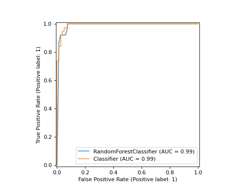
注意我们通过了 alpha=0.8 到绘图功能来调整曲线的Alpha值。
示例
sphx_glr_auto_examples_miscellaneous_plot_roc_curve_visualization_api.py
6.1. 可用的绘图实用程序#
6.1.1. 显示对象#
|
Calibration curve (also known as reliability diagram) visualization. |
|
部分依赖图(PDP)。 |
|
决策边界可视化。 |
|
混乱矩阵可视化。 |
|
DET曲线可视化。 |
|
精确召回可视化。 |
|
回归模型预测误差的可视化。 |
|
ROC曲线可视化。 |
学习曲线可视化。 |
|
验证曲线可视化。 |