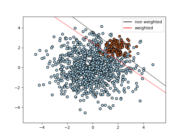
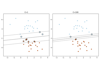
支持者：分离不平衡类别的超平面#

对于不平衡的类，使用SRC找到最佳分离超平面。

我们首先找到具有普通SRC的分离平面，然后绘制（虚线）具有不平衡类别自动纠正的分离超平面。

备注

此示例也将通过替换 SVC(kernel="linear") 与 SGDClassifier(loss="hinge") .设置 loss 参数 SGDClassifier 等于 hinge 将产生诸如具有线性内核的SVC的行为。

例如，尝试而不是 SVC

clf = SGDClassifier(n_iter=100, alpha=0.01)

# Authors: The scikit-learn developers
# SPDX-License-Identifier: BSD-3-Clause

import matplotlib.lines as mlines
import matplotlib.pyplot as plt

from sklearn import svm
from sklearn.datasets import make_blobs
from sklearn.inspection import DecisionBoundaryDisplay

# we create two clusters of random points
n_samples_1 = 1000
n_samples_2 = 100
centers = [[0.0, 0.0], [2.0, 2.0]]
clusters_std = [1.5, 0.5]
X, y = make_blobs(
    n_samples=[n_samples_1, n_samples_2],
    centers=centers,
    cluster_std=clusters_std,
    random_state=0,
    shuffle=False,
)

# fit the model and get the separating hyperplane
clf = svm.SVC(kernel="linear", C=1.0)
clf.fit(X, y)

# fit the model and get the separating hyperplane using weighted classes
wclf = svm.SVC(kernel="linear", class_weight={1: 10})
wclf.fit(X, y)

# plot the samples
plt.scatter(X[:, 0], X[:, 1], c=y, cmap=plt.cm.Paired, edgecolors="k")

# plot the decision functions for both classifiers
ax = plt.gca()
disp = DecisionBoundaryDisplay.from_estimator(
    clf,
    X,
    plot_method="contour",
    colors="k",
    levels=[0],
    alpha=0.5,
    linestyles=["-"],
    ax=ax,
)

# plot decision boundary and margins for weighted classes
wdisp = DecisionBoundaryDisplay.from_estimator(
    wclf,
    X,
    plot_method="contour",
    colors="r",
    levels=[0],
    alpha=0.5,
    linestyles=["-"],
    ax=ax,
)

plt.legend(
    [
        mlines.Line2D([], [], color="k", label="non weighted"),
        mlines.Line2D([], [], color="r", label="weighted"),
    ],
    ["non weighted", "weighted"],
    loc="upper right",
)
plt.show()

Total running time of the script: （0分0.116秒）