备注
Go to the end 下载完整的示例代码。或者通过浏览器中的MysterLite或Binder运行此示例
HDSCAN集群算法演示#
在这个演示中,我们将看看 cluster.HDBSCAN 从概括的角度来看 cluster.DBSCAN 算法我们将在特定数据集上比较这两种算法。最后,我们将评估HDSCAN对某些超参数的敏感性。
为了方便起见,我们首先定义几个效用函数。
# Authors: The scikit-learn developers
# SPDX-License-Identifier: BSD-3-Clause
import matplotlib.pyplot as plt
import numpy as np

from sklearn.cluster import DBSCAN, HDBSCAN
from sklearn.datasets import make_blobs


def plot(X, labels, probabilities=None, parameters=None, ground_truth=False, ax=None):
    if ax is None:
        _, ax = plt.subplots(figsize=(10, 4))
    labels = labels if labels is not None else np.ones(X.shape[0])
    probabilities = probabilities if probabilities is not None else np.ones(X.shape[0])
    # Black removed and is used for noise instead.
    unique_labels = set(labels)
    colors = [plt.cm.Spectral(each) for each in np.linspace(0, 1, len(unique_labels))]
    # The probability of a point belonging to its labeled cluster determines
    # the size of its marker
    proba_map = {idx: probabilities[idx] for idx in range(len(labels))}
    for k, col in zip(unique_labels, colors):
        if k == -1:
            # Black used for noise.
            col = [0, 0, 0, 1]

        class_index = (labels == k).nonzero()[0]
        for ci in class_index:
            ax.plot(
                X[ci, 0],
                X[ci, 1],
                "x" if k == -1 else "o",
                markerfacecolor=tuple(col),
                markeredgecolor="k",
                markersize=4 if k == -1 else 1 + 5 * proba_map[ci],
            )
    n_clusters_ = len(set(labels)) - (1 if -1 in labels else 0)
    preamble = "True" if ground_truth else "Estimated"
    title = f"{preamble} number of clusters: {n_clusters_}"
    if parameters is not None:
        parameters_str = ", ".join(f"{k}={v}" for k, v in parameters.items())
        title += f" | {parameters_str}"
    ax.set_title(title)
    plt.tight_layout()
生成示例数据#
HDSCAN相对于DBSCAN的最大优势之一是其开箱即用的稳健性。这对于异类数据混合来说尤其显着。与DBSCAN一样,它可以建模任意形状和分布,但与DBSCAN不同,它不需要任意且敏感的规范 eps 超参数
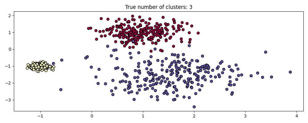
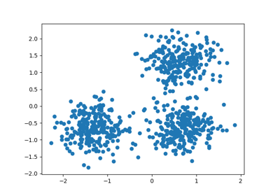
例如,下面我们从三个二维和各向同性高斯分布的混合中生成一个数据集。
centers = [[1, 1], [-1, -1], [1.5, -1.5]]
X, labels_true = make_blobs(
    n_samples=750, centers=centers, cluster_std=[0.4, 0.1, 0.75], random_state=0
)
plot(X, labels=labels_true, ground_truth=True)
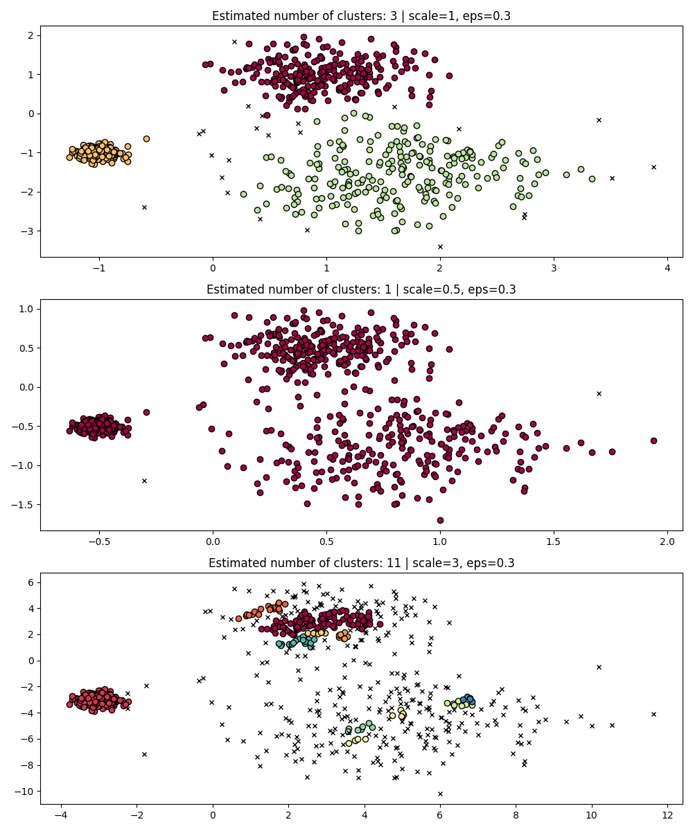
尺度不变性#
值得记住的是,虽然DBSCAN为 eps 参数时,它几乎没有合适的默认值,并且必须针对使用时的特定数据集进行调整。
作为一个简单的演示,考虑 eps 针对一个数据集调整值,并用相同的值获得集群,但应用于数据集的重新缩放版本。
fig, axes = plt.subplots(3, 1, figsize=(10, 12))
dbs = DBSCAN(eps=0.3)
for idx, scale in enumerate([1, 0.5, 3]):
    dbs.fit(X * scale)
    plot(X * scale, dbs.labels_, parameters={"scale": scale, "eps": 0.3}, ax=axes[idx])
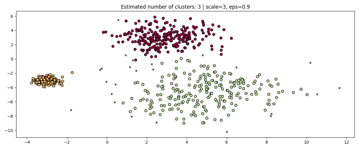
事实上,为了保持相同的结果,我们必须扩大规模 eps 同样的因素。
fig, axis = plt.subplots(1, 1, figsize=(12, 5))
dbs = DBSCAN(eps=0.9).fit(3 * X)
plot(3 * X, dbs.labels_, parameters={"scale": 3, "eps": 0.9}, ax=axis)
在标准化数据时(例如使用 sklearn.preprocessing.StandardScaler )有助于缓解这个问题,因此必须非常小心地选择合适的值 eps .
从这个意义上说,HDSCAN更加稳健:HDSCAN可以被视为对所有可能的值进行集群 eps 并从所有可能的集群中提取最佳集群(请参阅 User Guide ).一个直接的优势是HDSCAN是规模不变的。
fig, axes = plt.subplots(3, 1, figsize=(10, 12))
hdb = HDBSCAN()
for idx, scale in enumerate([1, 0.5, 3]):
    hdb.fit(X * scale)
    plot(
        X * scale,
        hdb.labels_,
        hdb.probabilities_,
        ax=axes[idx],
        parameters={"scale": scale},
    )

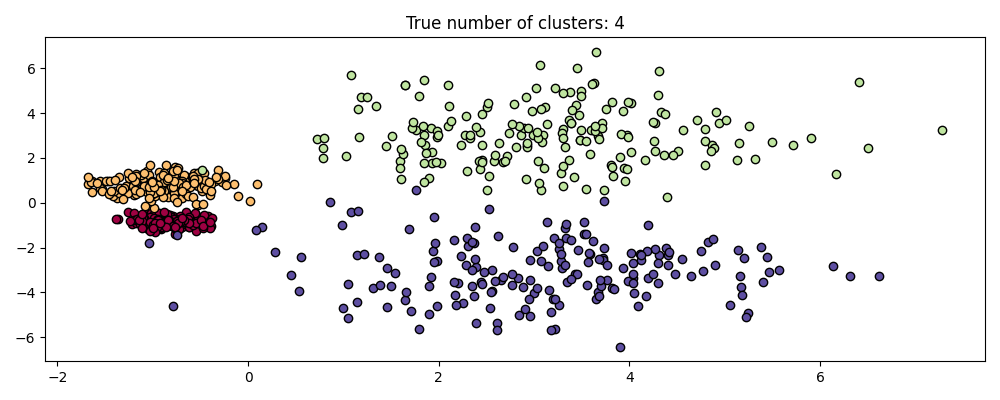
多尺度聚类#
不过,HDSCAN不仅仅是规模不变的--它能够进行多规模集群,这可以考虑不同密度的集群。传统的DBSCAN假设任何潜在的集群的密度都是均匀的。HDSCAN不受此类限制。为了证明这一点,我们考虑以下数据集
centers = [[-0.85, -0.85], [-0.85, 0.85], [3, 3], [3, -3]]
X, labels_true = make_blobs(
    n_samples=750, centers=centers, cluster_std=[0.2, 0.35, 1.35, 1.35], random_state=0
)
plot(X, labels=labels_true, ground_truth=True)
由于不同的密度和空间分离,该数据集对于DBSCAN来说更加困难:
如果
eps太大,那么我们就有可能错误地将两个密集的集群聚集为一个,因为它们的相互可达性将扩展集群。如果
eps太小,那么我们就有可能将较稀疏的集群分裂成许多虚假集群。
更不用说这需要手动调整选择 eps 直到我们找到一个我们满意的权衡。
fig, axes = plt.subplots(2, 1, figsize=(10, 8))
params = {"eps": 0.7}
dbs = DBSCAN(**params).fit(X)
plot(X, dbs.labels_, parameters=params, ax=axes[0])
params = {"eps": 0.3}
dbs = DBSCAN(**params).fit(X)
plot(X, dbs.labels_, parameters=params, ax=axes[1])
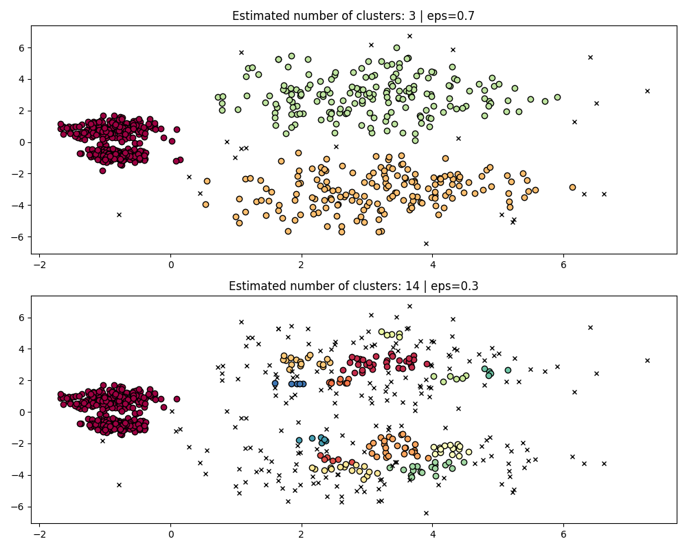
为了正确地聚集两个密集集群,我们需要较小的RST值,但是, eps=0.3 我们已经在碎片化稀疏集群,随着时间的减少,情况只会变得更加严重。事实上,DBSCAN似乎无法同时分离两个密集集群,同时防止稀疏集群碎片化。让我们与HDSCAN进行比较。
hdb = HDBSCAN().fit(X)
plot(X, hdb.labels_, hdb.probabilities_)
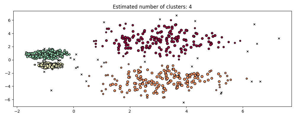
HDBSCAN能够适应数据集的多尺度结构,而无需参数调整。虽然任何足够有趣的数据集都需要调整,但这个案例表明,HDSCAN可以在没有用户干预的情况下产生质量上更好的集群类,而这些集群是通过DBSCAN无法访问的。
超参数鲁棒性#
最终,调整将是任何现实世界应用程序中的重要一步,因此让我们来看看HDBSCAN的一些最重要的超参数。虽然HDSCAN不受 eps DBSCAN的参数,它仍然有一些超参数,例如 min_cluster_size 和 min_samples 它调整了有关密度的结果。然而,我们将看到HDSCAN对于各种现实世界示例相对稳健,这要归功于这些参数,其含义明确有助于调整它们。
min_cluster_size#
min_cluster_size 是将该组视为集群的组中的最小样本数。
小于此大小的群集将作为噪声保留。默认值为5。此参数通常根据需要调整为较大的值。较小的值可能会导致结果中标记为噪声的点较少。然而,太小的值将导致错误的子集群被拾取和首选。对于有噪音的数据集,较大的值往往更稳健,例如具有显着重叠的高方差集群。
PARAM = ({"min_cluster_size": 5}, {"min_cluster_size": 3}, {"min_cluster_size": 25})
fig, axes = plt.subplots(3, 1, figsize=(10, 12))
for i, param in enumerate(PARAM):
    hdb = HDBSCAN(**param).fit(X)
    labels = hdb.labels_

    plot(X, labels, hdb.probabilities_, param, ax=axes[i])

min_samples#
min_samples 是被视为核心点的点(包括点本身)的邻近中的样本数。 min_samples 默认为 min_cluster_size .类似于 min_cluster_size ,更大的价值 min_samples 提高模型对噪音的鲁棒性,但有忽视或丢弃潜在有效但小的集群的风险。 min_samples 最好在找到一个很好的价值后进行调整 min_cluster_size .
PARAM = (
    {"min_cluster_size": 20, "min_samples": 5},
    {"min_cluster_size": 20, "min_samples": 3},
    {"min_cluster_size": 20, "min_samples": 25},
)
fig, axes = plt.subplots(3, 1, figsize=(10, 12))
for i, param in enumerate(PARAM):
    hdb = HDBSCAN(**param).fit(X)
    labels = hdb.labels_

    plot(X, labels, hdb.probabilities_, param, ax=axes[i])

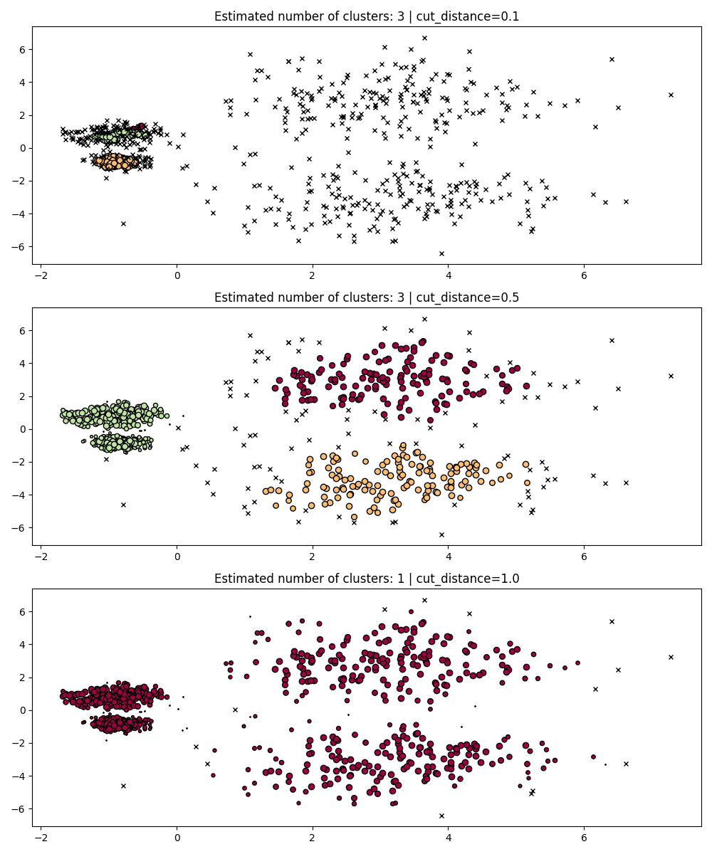
dbscan_clustering#
期间 fit , HDBSCAN 构建一个单一的链接树,该树对所有值上的所有点的聚类进行编码, DBSCAN 的 eps 参数.因此,我们可以有效地绘制和评估这些集群,而无需完全重新计算中间值,例如核心距离、互达性和最小生成树。我们需要做的就是指定 cut_distance (相当于 eps )我们想要集群。
PARAM = (
    {"cut_distance": 0.1},
    {"cut_distance": 0.5},
    {"cut_distance": 1.0},
)
hdb = HDBSCAN()
hdb.fit(X)
fig, axes = plt.subplots(len(PARAM), 1, figsize=(10, 12))
for i, param in enumerate(PARAM):
    labels = hdb.dbscan_clustering(**param)

    plot(X, labels, hdb.probabilities_, param, ax=axes[i])
Total running time of the script: (0分9.829秒)
相关实例
Gallery generated by Sphinx-Gallery <https://sphinx-gallery.github.io> _