>>> from env_helper import info; info()
页面更新时间: 2023-06-24 12:25:58
运行环境:
    Linux发行版本: Debian GNU/Linux 12 (bookworm)
    操作系统内核: Linux-6.1.0-9-amd64-x86_64-with-glibc2.36
    Python版本: 3.11.2
2.3. Python数字图像处理:图像简单滤波
对图像进行滤波,可以有两种效果:一种是平滑滤波,用来抑制噪声;另一种是微分算子,可以用来检测边缘和特征提取。
skimage库中通过filters模块进行滤波操作。
2.3.1. sobel算子
sobel算子可用来检测边缘
函数格式为: skimage.filters.sobel(image, mask=None)
>>> from skimage import data,filters
>>> import matplotlib.pyplot as plt
>>> img = data.camera()
>>> edges = filters.sobel(img)
>>> plt.imshow(edges,plt.cm.gray)
<matplotlib.image.AxesImage at 0x7f989e66d810>

2.3.2. roberts算子
roberts算子和sobel算子一样,用于检测边缘
调用格式也是一样的:
>>> edges = filters.roberts(img)
>>> plt.imshow(edges,plt.cm.gray)
<matplotlib.image.AxesImage at 0x7f989dafeb10>
2.3.3. scharr算子
功能同sobel,调用格式:
>>> edges = filters.scharr(img)
>>> plt.imshow(edges,plt.cm.gray)
<matplotlib.image.AxesImage at 0x7f989db70410>

2.3.4. prewitt算子
功能同sobel,调用格式:
>>> edges = filters.prewitt(img)
>>> plt.imshow(edges,plt.cm.gray)
<matplotlib.image.AxesImage at 0x7f989dbce590>
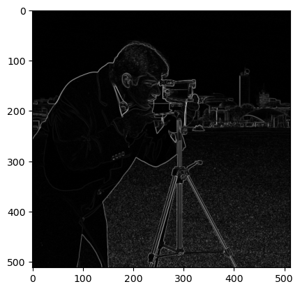
2.3.5. canny算子
canny算子也是用于提取边缘特征,但它不是放在filters模块,而是放在feature模块
函数格式:skimage.feature.canny(image,sigma=1.0)
可以修改sigma的值来调整效果
>>> from skimage import data,filters,feature
>>> import matplotlib.pyplot as plt
>>> img = data.camera()
>>> edges1 = feature.canny(img)   #sigma=1
>>> edges2 = feature.canny(img,sigma=3)   #sigma=3
>>>
>>> plt.figure('canny',figsize=(8,8))
>>> plt.subplot(121)
>>> plt.imshow(edges1,plt.cm.gray)
>>>
>>> plt.subplot(122)
>>> plt.imshow(edges2,plt.cm.gray)
>>>
>>> plt.show()
从结果可以看出,sigma越小,边缘线条越细小。
2.3.6. gabor滤波
gabor滤波可用来进行边缘检测和纹理特征提取。
函数调用格式:skimage.filters.gabor(image, frequency) skimage.filters.gabor_filter(图片,频率)弃用功能。改为使用skimage.filters.gabor。
通过修改frequency值来调整滤波效果,返回一对边缘结果,一个是用真实滤波核的滤波结果,一个是想象的滤波核的滤波结果。
>>> from skimage import data,filters
>>> import matplotlib.pyplot as plt
>>> img = data.camera()
>>> filt_real, filt_imag = filters.gabor(img,frequency=0.6)
>>>
>>> plt.figure('gabor',figsize=(8,8))
>>>
>>> plt.subplot(121)
>>> plt.title('filt_real')
>>> plt.imshow(filt_real,plt.cm.gray)
>>>
>>> plt.subplot(122)
>>> plt.title('filt-imag')
>>> plt.imshow(filt_imag,plt.cm.gray)
>>>
>>> plt.show()
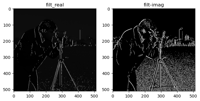
以上为frequency=0.6的结果图。
>>> filt_real, filt_imag = filters.gabor(img,frequency=0.1)
>>>
>>> plt.figure('gabor',figsize=(8,8))
>>>
>>> plt.subplot(121)
>>> plt.title('filt_real')
>>> plt.imshow(filt_real,plt.cm.gray)
>>>
>>> plt.subplot(122)
>>> plt.title('filt-imag')
>>> plt.imshow(filt_imag,plt.cm.gray)
>>>
>>> plt.show()
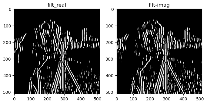
以上为frequency=0.1的结果图
2.3.7. gaussian滤波
多维的滤波器,是一种平滑滤波,可以消除高斯噪声。
调用函数为:skimage.filters.gaussian(image, sigma) skimage.filters.gaussian_filter(image,…)弃用功能。改为使用skimage.filters.gaussian。
通过调节sigma的值来调整滤波效果
>>> from skimage import data,filters
>>> import matplotlib.pyplot as plt
>>> img = data.astronaut()
>>> edges1 = filters.gaussian(img,sigma=0.4)   #sigma=0.4
>>> edges2 = filters.gaussian(img,sigma=5)   #sigma=5
>>>
>>> plt.figure('gaussian',figsize=(8,8))
>>> plt.subplot(121)
>>> plt.imshow(edges1,plt.cm.gray)
>>>
>>> plt.subplot(122)
>>> plt.imshow(edges2,plt.cm.gray)
>>>
>>> plt.show()
/usr/lib/python3/dist-packages/skimage/_shared/utils.py:348: RuntimeWarning: Images with dimensions (M, N, 3) are interpreted as 2D+RGB by default. Use multichannel=False to interpret as 3D image with last dimension of length 3.
  return func(*args, **kwargs)
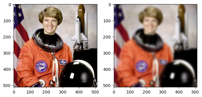
可见sigma越大,过滤后的图像越模糊
2.3.8. median
中值滤波,一种平滑滤波,可以消除噪声。
需要用skimage.morphology模块来设置滤波器的形状。
>>> from skimage import data,filters
>>> import matplotlib.pyplot as plt
>>> from skimage.morphology import disk
>>> img = data.camera()
>>> edges1 = filters.median(img,disk(5))
>>> edges2= filters.median(img,disk(9))
>>>
>>> plt.figure('median',figsize=(8,8))
>>>
>>> plt.subplot(121)
>>> plt.imshow(edges1,plt.cm.gray)
>>>
>>> plt.subplot(122)
>>> plt.imshow(edges2,plt.cm.gray)
>>>
>>> plt.show()
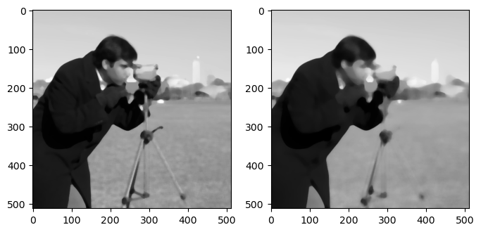
从结果可以看出,滤波器越大,图像越模糊。
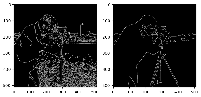
2.3.9. 水平、垂直边缘检测
上边所举的例子都是进行全部边缘检测,有些时候我们只需要检测水平边缘,或垂直边缘,就可用下面的方法。
水平边缘检测: sobel_h , prewitt_h , scharr_h
垂直边缘检测: sobel_v , prewitt_v , scharr_v
>>> from skimage import data,filters
>>> import matplotlib.pyplot as plt
>>> img = data.camera()
>>> edges1 = filters.sobel_h(img)
>>> edges2 = filters.sobel_v(img)
>>>
>>> plt.figure('sobel_v_h',figsize=(8,8))
>>>
>>> plt.subplot(121)
>>> plt.imshow(edges1,plt.cm.gray)
>>>
>>> plt.subplot(122)
>>> plt.imshow(edges2,plt.cm.gray)
>>>
>>> plt.show()
上边左图为检测出的水平边缘,右图为检测出的垂直边缘。
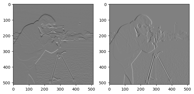
2.3.10. 交叉边缘检测
可使用Roberts的十字交叉核来进行过滤,以达到检测交叉边缘的目的。这些交叉边缘实际上是梯度在某个方向上的一个分量。
其中一个核:
 0   1
-1   0
对应的函数:
roberts_neg_diag(image)
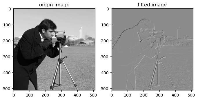
例:
>>> import matplotlib.pyplot as plt
>>> img =data.camera()
>>> dst =filters.roberts_neg_diag(img)
>>>
>>> plt.figure('filters',figsize=(8,8))
>>> plt.subplot(121)
>>> plt.title('origin image')
>>> plt.imshow(img,plt.cm.gray)
>>>
>>> plt.subplot(122)
>>> plt.title('filted image')
>>> plt.imshow(dst,plt.cm.gray)
<matplotlib.image.AxesImage at 0x7f9897481a50>
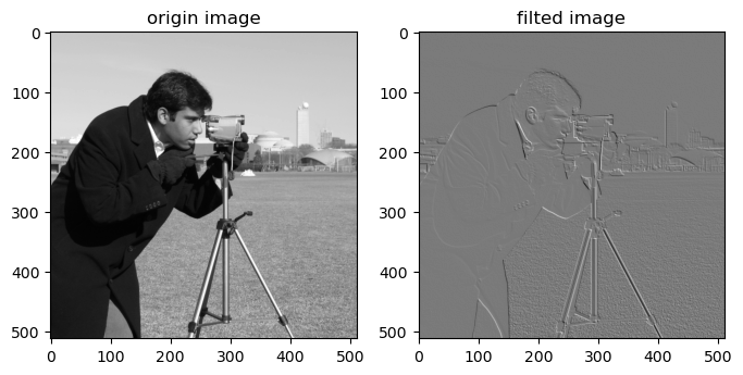
另外一个核:
1   0
0  -1
对应函数为:
roberts_pos_diag(image)
>>> import matplotlib.pyplot as plt
>>> img =data.camera()
>>> dst =filters.roberts_pos_diag(img)
>>>
>>> plt.figure('filters',figsize=(8,8))
>>> plt.subplot(121)
>>> plt.title('origin image')
>>> plt.imshow(img,plt.cm.gray)
>>>
>>> plt.subplot(122)
>>> plt.title('filted image')
>>> plt.imshow(dst,plt.cm.gray)
<matplotlib.image.AxesImage at 0x7f989749d010>