3.4. Python数字图像处理(17):边缘与轮廓
在前面的python数字图像处理(10):图像简单滤波 中,我们已经讲解了很多算子用来检测边缘,其中用得最多的canny算子边缘检测。
本篇我们讲解一些其它方法来检测轮廓。
3.4.1. 查找轮廓(find_contours)
measure模块中的find_contours()函数,可用来检测二值图像的边缘轮廓。
函数原型为:
skimage.measure.find_contours(array, level)
array: 一个二值数组图像
level: 在图像中查找轮廓的级别值
返回轮廓列表集合,可用for循环取出每一条轮廓。
例1:
>>> import numpy as np
>>> import matplotlib.pyplot as plt
>>> from skimage import measure,draw
>>>
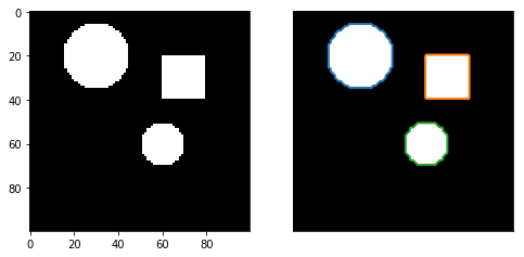
>>> #生成二值测试图像
>>> img=np.zeros([100,100])
>>> img[20:40,60:80]=1 #矩形
>>> rr,cc=draw.circle(60,60,10) #小圆
>>> rr1,cc1=draw.circle(20,30,15) #大圆
>>> img[rr,cc]=1
>>> img[rr1,cc1]=1
>>>
>>> #检测所有图形的轮廓
>>> contours = measure.find_contours(img, 0.5)
>>>
>>> #绘制轮廓
>>> fig, (ax0,ax1) = plt.subplots(1,2,figsize=(8,8))
>>> ax0.imshow(img,plt.cm.gray)
>>> ax1.imshow(img,plt.cm.gray)
>>> for n, contour in enumerate(contours):
>>> ax1.plot(contour[:, 1], contour[:, 0], linewidth=2)
>>> ax1.axis('image')
>>> ax1.set_xticks([])
>>> ax1.set_yticks([])
>>> plt.show()
>>>
>>> #结果如下:不同的轮廓用不同的颜色显示
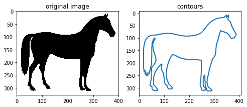
例2:
>>> import matplotlib.pyplot as plt
>>> from skimage import measure,data,color
>>>
>>> #生成二值测试图像
>>> img=color.rgb2gray(data.horse())
>>>
>>> #检测所有图形的轮廓
>>> contours = measure.find_contours(img, 0.5)
>>>
>>> #绘制轮廓
>>> fig, axes = plt.subplots(1,2,figsize=(8,8))
>>> ax0, ax1= axes.ravel()
>>> ax0.imshow(img,plt.cm.gray)
>>> ax0.set_title('original image')
>>>
>>> rows,cols=img.shape
>>> ax1.axis([0,rows,cols,0])
>>> for n, contour in enumerate(contours):
>>>     ax1.plot(contour[:, 1], contour[:, 0], linewidth=2)
>>> ax1.axis('image')
>>> ax1.set_title('contours')
>>> plt.show()
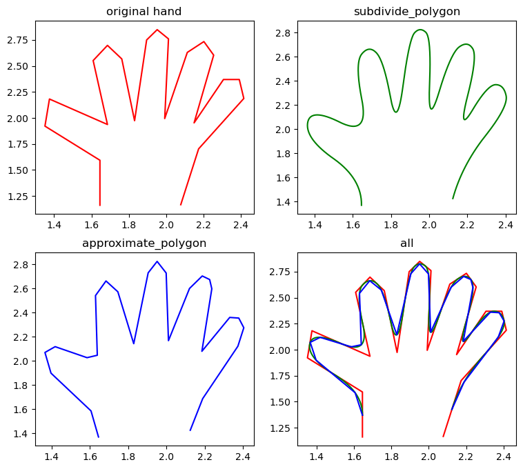
3.4.2. 逼近多边形曲线
逼近多边形曲线有两个函数: subdivide_polygon() 和
approximate_polygon()
subdivide_polygon()
采用B样条(B-Splines)来细分多边形的曲线,该曲线通常在凸包线的内部。
函数格式为:
skimage.measure.subdivide_polygon(coords, degree=2, preserve_ends=False)
coords: 坐标点序列。degree: B样条的度数,默认为2preserve_ends: 如果曲线为非闭合曲线,是否保存开始和结束点坐标,默认为False
返回细分为的坐标点序列。
approximate_polygon() 是基于Douglas-Peucker算法的一种近似曲线模拟。
它根据指定的容忍值来近似一条多边形曲线链,该曲线也在凸包线的内部。
函数格式为:
skimage.measure.approximate_polygon(coords, tolerance)
coords: 坐标点序列tolerance: 容限值
返回近似的多边形曲线坐标序列。
例:
>>> import numpy as np
>>> import matplotlib.pyplot as plt
>>> from skimage import measure,data,color
生成二值测试图像:
>>> hand = np.array([[1.64516129, 1.16145833],
>>>                  [1.64516129, 1.59375],
>>>                  [1.35080645, 1.921875],
>>>                  [1.375, 2.18229167],
>>>                  [1.68548387, 1.9375],
>>>                  [1.60887097, 2.55208333],
>>>                  [1.68548387, 2.69791667],
>>>                  [1.76209677, 2.56770833],
>>>                  [1.83064516, 1.97395833],
>>>                  [1.89516129, 2.75],
>>>                  [1.9516129, 2.84895833],
>>>                  [2.01209677, 2.76041667],
>>>                  [1.99193548, 1.99479167],
>>>                  [2.11290323, 2.63020833],
>>>                  [2.2016129, 2.734375],
>>>                  [2.25403226, 2.60416667],
>>>                  [2.14919355, 1.953125],
>>>                  [2.30645161, 2.36979167],
>>>                  [2.39112903, 2.36979167],
>>>                  [2.41532258, 2.1875],
>>>                  [2.1733871, 1.703125],
>>>                  [2.07782258, 1.16666667]])
检测所有图形的轮廓:
>>> new_hand = hand.copy()
>>> for _ in range(5):
>>>     new_hand =measure.subdivide_polygon(new_hand, degree=2)
approximate subdivided polygon with Douglas-Peucker algorithm:
>>> appr_hand =measure.approximate_polygon(new_hand, tolerance=0.02)
>>>
>>> print("Number of coordinates:", len(hand), len(new_hand), len(appr_hand))
>>>
>>> fig, axes= plt.subplots(2,2, figsize=(9, 8))
>>> ax0,ax1,ax2,ax3=axes.ravel()
>>>
>>> ax0.plot(hand[:, 0], hand[:, 1],'r')
>>> ax0.set_title('original hand')
>>> ax1.plot(new_hand[:, 0], new_hand[:, 1],'g')
>>> ax1.set_title('subdivide_polygon')
>>> ax2.plot(appr_hand[:, 0], appr_hand[:, 1],'b')
>>> ax2.set_title('approximate_polygon')
>>>
>>> ax3.plot(hand[:, 0], hand[:, 1],'r')
>>> ax3.plot(new_hand[:, 0], new_hand[:, 1],'g')
>>> ax3.plot(appr_hand[:, 0], appr_hand[:, 1],'b')
>>> ax3.set_title('all')
Number of coordinates: 22 642 26
Text(0.5, 1.0, 'all')