作图#
介绍#
The plotting module allows you to make 2-dimensional and 3-dimensional plots.
Presently the plots are rendered using matplotlib as a
backend. It is also possible to plot 2-dimensional plots using a
TextBackend if you do not have matplotlib.
绘图模块具有以下功能:
plot(): Plots 2D line plots.plot_parametric(): Plots 2D parametric plots.plot_implicit(): Plots 2D implicit and region plots.plot3d(): Plots 3D plots of functions in two variables.plot3d_parametric_line(): Plots 3D line plots, defined by a parameter.plot3d_parametric_surface(): Plots 3D parametric surface plots.
The above functions are only for convenience and ease of use. It is possible to
plot any plot by passing the corresponding Series class to Plot as
argument.
绘图类#
- class sympy.plotting.plot.Plot(*args, title=None, xlabel=None, ylabel=None, zlabel=None, aspect_ratio='auto', xlim=None, ylim=None, axis_center='auto', axis=True, xscale='linear', yscale='linear', legend=False, autoscale=True, margin=0, annotations=None, markers=None, rectangles=None, fill=None, backend='default', size=None, **kwargs)[源代码]#
所有后端的基类。后端表示打印库,它实现了使用SymPy打印函数所需的功能。
For interactive work the function
plot()is better suited.This class permits the plotting of SymPy expressions using numerous backends (
matplotlib, textplot, the old pyglet module for SymPy, Google charts api, etc).The figure can contain an arbitrary number of plots of SymPy expressions, lists of coordinates of points, etc. Plot has a private attribute _series that contains all data series to be plotted (expressions for lines or surfaces, lists of points, etc (all subclasses of BaseSeries)). Those data series are instances of classes not imported by
from sympy import *.The customization of the figure is on two levels. Global options that concern the figure as a whole (e.g. title, xlabel, scale, etc) and per-data series options (e.g. name) and aesthetics (e.g. color, point shape, line type, etc.).
The difference between options and aesthetics is that an aesthetic can be a function of the coordinates (or parameters in a parametric plot). The supported values for an aesthetic are:
None (the backend uses default values)
a constant
a function of one variable (the first coordinate or parameter)
a function of two variables (the first and second coordinate or parameters)
a function of three variables (only in nonparametric 3D plots)
Their implementation depends on the backend so they may not work in some backends.
如果情节是参数化的,并且审美功能的数量允许它,那么美感是在参数上而不是在坐标上计算的。如果arity不允许对参数进行计算,则在坐标上进行计算。
目前只支持笛卡尔坐标,但可以使用参数化绘图以极坐标、球坐标和柱坐标进行打印。
构造函数绘图的参数必须是BaseSeries的子类。
任何全局选项都可以指定为关键字参数。
图形的全局选项包括:
标题:str
xlabel : str or Symbol
ylabel : str or Symbol
zlabel : str or Symbol
传说:布尔
xscale:{'linear','log'}
yscale:{'linear','log'}
轴:bool
axis_center:两个float的元组或{'center','auto'}
xlim:两个浮点数的元组
ylim:两个浮点数的元组
纵横比:两个浮点的元组或{'auto'}
自动缩放:布尔
边距:浮动 [0, 1]
后端:{'default'、'matplotlib'、'text'}或BaseBackend的子类
大小:两个浮点的可选元组,(宽度,高度);默认值:无
每个数据系列的选项和美感是:基本系列中没有。有关子类,请参见下面的选项。
一些数据系列支持其他美学或选项:
LineOver1DRangeSeries,Parametric2DLineSeries, andParametric3DLineSeriessupport the following:美学:
- line_colorstring, or float, or function, optional
Specifies the color for the plot, which depends on the backend being used.
For example, if
MatplotlibBackendis being used, then Matplotlib string colors are acceptable ("red","r","cyan","c", ...). Alternatively, we can use a float number, 0 < color < 1, wrapped in a string (for example,line_color="0.5") to specify grayscale colors. Alternatively, We can specify a function returning a single float value: this will be used to apply a color-loop (for example,line_color=lambda x: math.cos(x)).Note that by setting line_color, it would be applied simultaneously to all the series.
Options:
标签:str
步骤:布尔
仅限整数:bool
SurfaceOver2DRangeSeriesandParametricSurfaceSeriessupport the following:美学:
返回一个float:u函数。
笔记
绘图模块的工作原理:
Whenever a plotting function is called, the provided expressions are processed and a list of instances of the
BaseSeriesclass is created, containing the necessary information to plot the expressions (e.g. the expression, ranges, series name, ...). Eventually, these objects will generate the numerical data to be plotted.A subclass of
Plotclass is instantiaed (referred to as backend, from now on), which stores the list of series and the main attributes of the plot (e.g. axis labels, title, ...). The backend implements the logic to generate the actual figure with some plotting library.When the
showcommand is executed, series are processed one by one to generate numerical data and add it to the figure. The backend is also going to set the axis labels, title, ..., according to the values stored in the Plot instance.
The backend should check if it supports the data series that it is given (e.g.
TextBackendsupports onlyLineOver1DRangeSeries).It is the backend responsibility to know how to use the class of data series that it's given. Note that the current implementation of the
*Seriesclasses is "matplotlib-centric": the numerical data returned by theget_pointsandget_meshesmethods is meant to be used directly by Matplotlib. Therefore, the new backend will have to pre-process the numerical data to make it compatible with the chosen plotting library. Keep in mind that future SymPy versions may improve the*Seriesclasses in order to return numerical data "non-matplotlib-centric", hence if you code a new backend you have the responsibility to check if its working on each SymPy release.Please explore the
MatplotlibBackendsource code to understand how a backend should be coded.In order to be used by SymPy plotting functions, a backend must implement the following methods:
- show(self): used to loop over the data series, generate the numerical
data, plot it and set the axis labels, title, ...
- save(self, path): used to save the current plot to the specified file
path.
- close(self): used to close the current plot backend (note: some plotting
library does not support this functionality. In that case, just raise a warning).
- property annotations#
自 1.13 版本弃用.
- append(arg)[源代码]#
将绘图系列中的元素添加到现有绘图中。
实例
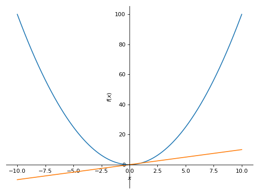
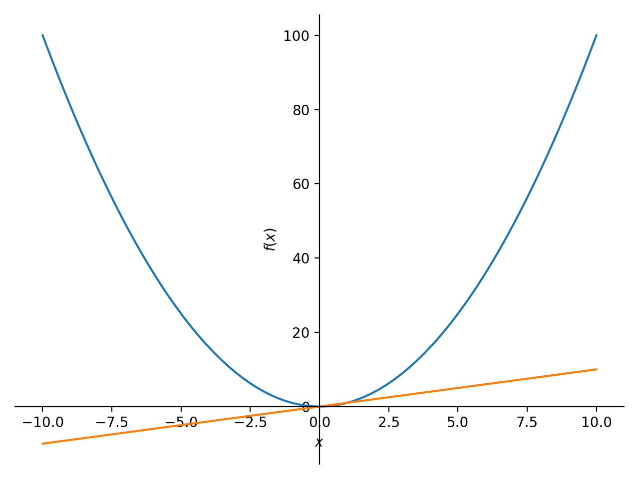
考虑两个
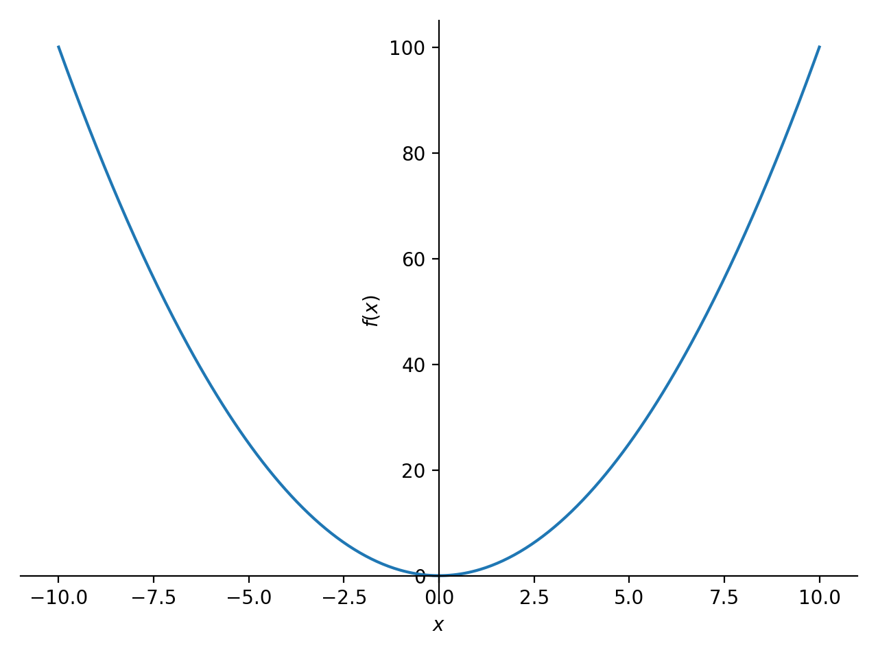
Plot物体,p1和p2. 要将第二个绘图的第一个系列对象添加到第一个,请使用append方法如下:>>> from sympy import symbols >>> from sympy.plotting import plot >>> x = symbols('x') >>> p1 = plot(x*x, show=False) >>> p2 = plot(x, show=False) >>> p1.append(p2[0]) >>> p1 Plot object containing: [0]: cartesian line: x**2 for x over (-10.0, 10.0) [1]: cartesian line: x for x over (-10.0, 10.0) >>> p1.show()
参见
- extend(arg)[源代码]#
添加其他绘图中的所有系列。
实例
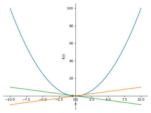
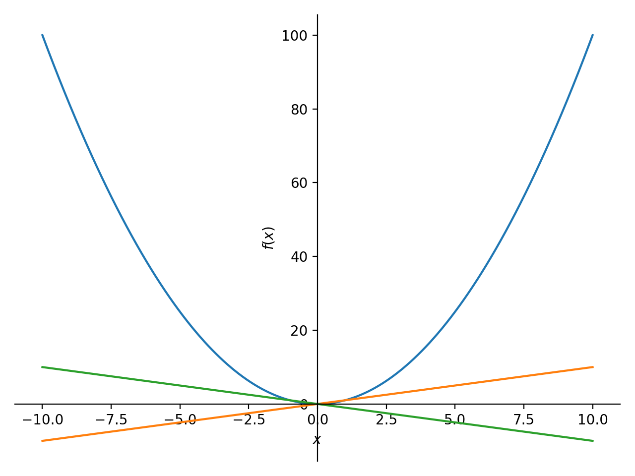
考虑两个
Plot物体,p1和p2. 要将第二个绘图添加到第一个绘图,请使用extend方法如下:>>> from sympy import symbols >>> from sympy.plotting import plot >>> x = symbols('x') >>> p1 = plot(x**2, show=False) >>> p2 = plot(x, -x, show=False) >>> p1.extend(p2) >>> p1 Plot object containing: [0]: cartesian line: x**2 for x over (-10.0, 10.0) [1]: cartesian line: x for x over (-10.0, 10.0) [2]: cartesian line: -x for x over (-10.0, 10.0) >>> p1.show()

- property fill#
自 1.13 版本弃用.
- property markers#
自 1.13 版本弃用.
- property rectangles#
自 1.13 版本弃用.
绘图功能参考#
- sympy.plotting.plot.plot(*args, show=True, **kwargs)[源代码]#
将单个变量的函数绘制为曲线。
- 参数:
args :
第一个参数是表示要绘制的单变量函数的表达式。
最后一个参数是表示自由变量范围的3元组。例如
(x, 0, 5)Typical usage examples are in the following:
- 绘制具有单个范围的单个表达式。
plot(expr, range, **kwargs)
- 使用默认范围(-10,10)打印单个表达式。
plot(expr, **kwargs)
- 用一个范围打印多个表达式。
plot(expr1, expr2, ..., range, **kwargs)
- 打印具有多个范围的多个表达式。
plot((expr1, range1), (expr2, range2), ..., **kwargs)
最好是显式地指定范围,因为如果实现更高级的默认范围检测算法,默认范围将来可能会更改。
show :bool,可选
默认值设置为
True. 将显示设置为False函数不会显示绘图。的返回实例Plot类可以通过调用save()和show()方法分别为。line_color : string, or float, or function, optional
Specifies the color for the plot. See
Plotto see how to set color for the plots. Note that by settingline_color, it would be applied simultaneously to all the series.标题 :str,可选
地块的标题。如果绘图只有一个表达式,则将其设置为表达式的 Latex 表示形式。
标签 :str,可选
表达式中的标签。它将在调用时使用
legend. 默认值是表达式的名称。例如sin(x)xlabel : str or expression, optional
x轴的标签。
ylabel : str or expression, optional
y轴的标签。
X标度 :“linear”或“log”,可选
设置x轴的缩放比例。
大比例尺 :“linear”或“log”,可选
设置y轴的缩放比例。
axis_center :(浮动,浮动),可选
两个浮点数的元组,表示中心或{'center','auto'}
xlim :(浮动,浮动),可选
表示x轴极限,
(min, max)'.ylim :(浮动,浮动),可选
表示y轴限制,
(min, max)'.注解 :列表,可选
A list of dictionaries specifying the type of annotation required. The keys in the dictionary should be equivalent to the arguments of the
matplotlib'sannotate()method.标记 :列表,可选
A list of dictionaries specifying the type the markers required. The keys in the dictionary should be equivalent to the arguments of the
matplotlib'splot()function along with the marker related keyworded arguments.矩形 :列表,可选
A list of dictionaries specifying the dimensions of the rectangles to be plotted. The keys in the dictionary should be equivalent to the arguments of the
matplotlib'sRectangleclass.fill :dict,可选
A dictionary specifying the type of color filling required in the plot. The keys in the dictionary should be equivalent to the arguments of the
matplotlib'sfill_between()method.适应的 :bool,可选
The default value is set to
True. Set adaptive toFalseand specifynif uniform sampling is required.绘图使用一种自适应算法,递归采样以精确绘图。自适应算法在两个点的中点附近使用一个随机点,该点必须进一步采样。因此,相同的情节可能会略有不同。
深度 :int,可选
Recursion depth of the adaptive algorithm. A depth of value \(n\) samples a maximum of \(2^{n}\) points.
如果
adaptive标志设置为False,这将被忽略。n : int, optional
Used when the
adaptiveis set toFalse. The function is uniformly sampled atnnumber of points. If theadaptiveflag is set toTrue, this will be ignored. This keyword argument replacesnb_of_points, which should be considered deprecated.size :(浮动,浮动),可选
以英寸为单位的形式(宽度、高度)的元组,用于指定整个图形的大小。默认值设置为
None,这意味着大小将由默认后端设置。
实例
>>> from sympy import symbols
>>> from sympy.plotting import plot
>>> x = symbols('x')
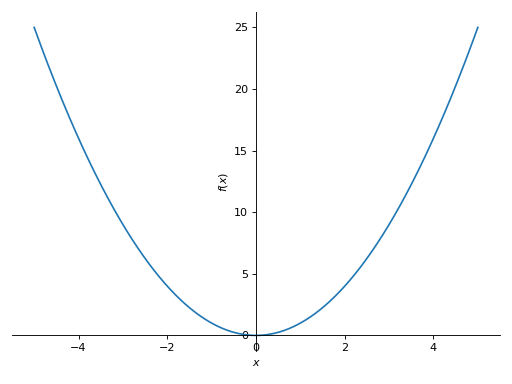
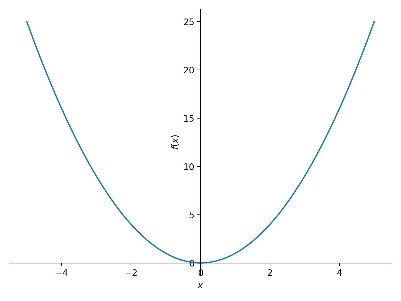
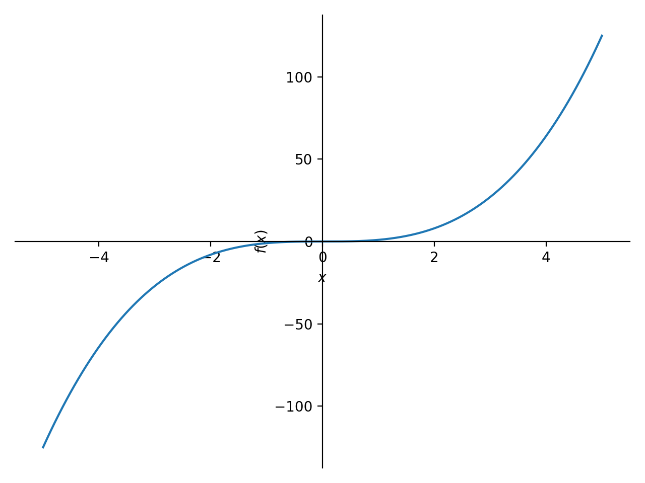
单一地块
>>> plot(x**2, (x, -5, 5))
Plot object containing:
[0]: cartesian line: x**2 for x over (-5.0, 5.0)
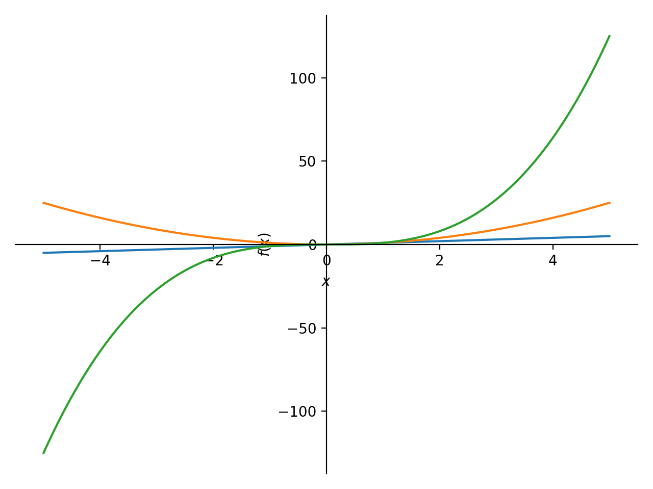
单一范围的多个绘图。
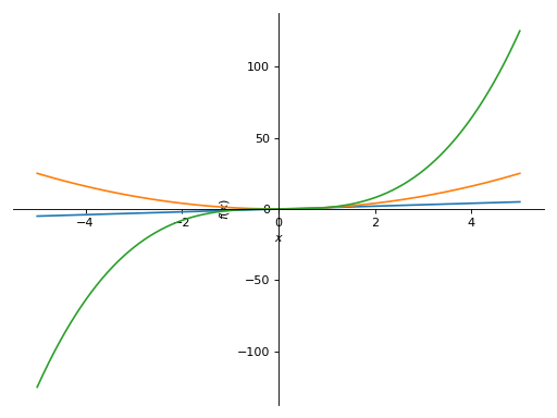
>>> plot(x, x**2, x**3, (x, -5, 5))
Plot object containing:
[0]: cartesian line: x for x over (-5.0, 5.0)
[1]: cartesian line: x**2 for x over (-5.0, 5.0)
[2]: cartesian line: x**3 for x over (-5.0, 5.0)

具有不同范围的多个绘图。
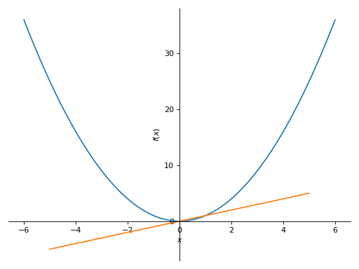
>>> plot((x**2, (x, -6, 6)), (x, (x, -5, 5)))
Plot object containing:
[0]: cartesian line: x**2 for x over (-6.0, 6.0)
[1]: cartesian line: x for x over (-5.0, 5.0)

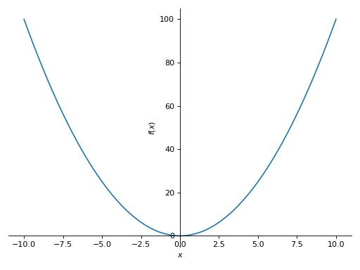
无自适应采样。
>>> plot(x**2, adaptive=False, n=400)
Plot object containing:
[0]: cartesian line: x**2 for x over (-10.0, 10.0)

- sympy.plotting.plot.plot_parametric(*args, show=True, **kwargs)[源代码]#
打印二维参数曲线。
- 参数:
args
常见规格为:
- 绘制具有范围的单参数曲线
plot_parametric((expr_x, expr_y), range)
- 绘制具有相同范围的多条参数曲线
plot_parametric((expr_x, expr_y), ..., range)
- 绘制具有不同范围的多条参数曲线
plot_parametric((expr_x, expr_y, range), ...)
expr_x表示参数函数的\(x\)组件的表达式。expr_y表示参数函数的\(y\)组件的表达式。range是一个三元组,表示参数符号start和stop。例如,(u, 0, 5).如果未指定范围,则使用默认范围(-10,10)。
但是,如果参数指定为
(expr_x, expr_y, range), ...,必须手动指定每个表达式的范围。如果实现更高级的算法,默认范围将来可能会改变。
适应的 :bool,可选
指定是否使用自适应采样。
The default value is set to
True. Set adaptive toFalseand specifynif uniform sampling is required.深度 :int,可选
自适应算法的递归深度。值为\(n\)的深度最多可采样\(2^n\)个点。
n : int, optional
Used when the
adaptiveflag is set toFalse. Specifies the number of the points used for the uniform sampling. This keyword argument replacesnb_of_points, which should be considered deprecated.line_color : string, or float, or function, optional
Specifies the color for the plot. See
Plotto see how to set color for the plots. Note that by settingline_color, it would be applied simultaneously to all the series.标签 :str,可选
表达式中的标签。它将在调用时使用
legend. 默认值是表达式的名称。例如sin(x)XLAP :str,可选
x轴的标签。
YLable :str,可选
y轴的标签。
X标度 :“linear”或“log”,可选
设置x轴的缩放比例。
大比例尺 :“linear”或“log”,可选
设置y轴的缩放比例。
axis_center :(浮动,浮动),可选
两个浮点数的元组,表示中心或{'center','auto'}
xlim :(浮动,浮动),可选
表示x轴极限,
(min, max)'.ylim :(浮动,浮动),可选
表示y轴限制,
(min, max)'.size :(浮动,浮动),可选
以英寸为单位的形式(宽度、高度)的元组,用于指定整个图形的大小。默认值设置为
None,这意味着大小将由默认后端设置。
实例
>>> from sympy import plot_parametric, symbols, cos, sin
>>> u = symbols('u')
带有单个表达式的参数化绘图:
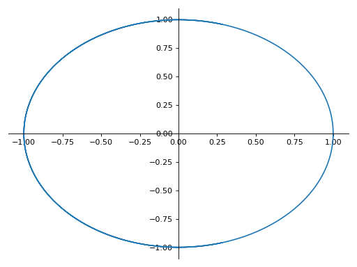
>>> plot_parametric((cos(u), sin(u)), (u, -5, 5))
Plot object containing:
[0]: parametric cartesian line: (cos(u), sin(u)) for u over (-5.0, 5.0)

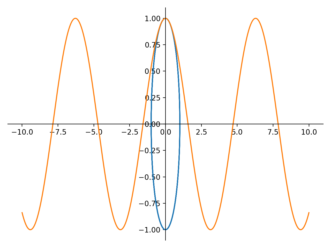
具有相同范围的多个表达式的参数化打印:
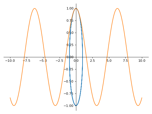
>>> plot_parametric((cos(u), sin(u)), (u, cos(u)), (u, -10, 10))
Plot object containing:
[0]: parametric cartesian line: (cos(u), sin(u)) for u over (-10.0, 10.0)
[1]: parametric cartesian line: (u, cos(u)) for u over (-10.0, 10.0)

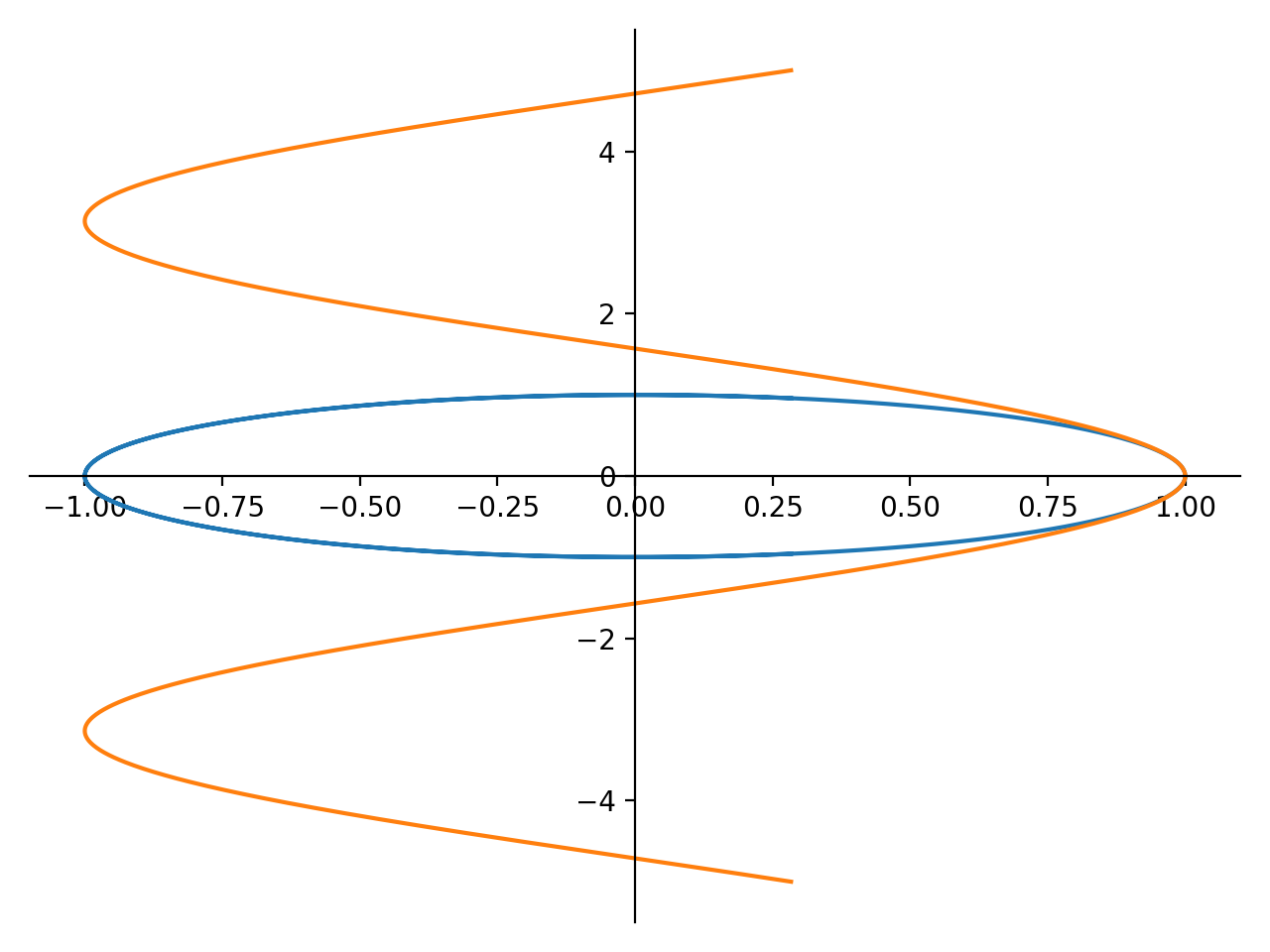
带有多个表达式的参数化绘图,每个曲线的范围不同:
>>> plot_parametric((cos(u), sin(u), (u, -5, 5)),
...     (cos(u), u, (u, -5, 5)))
Plot object containing:
[0]: parametric cartesian line: (cos(u), sin(u)) for u over (-5.0, 5.0)
[1]: parametric cartesian line: (cos(u), u) for u over (-5.0, 5.0)

笔记
绘图使用自适应算法,递归采样,以精确绘制曲线。自适应算法在两个点的中点附近使用一个随机点,该点必须进一步采样。因此,由于随机采样,重复相同的plot命令可能会得到稍微不同的结果。
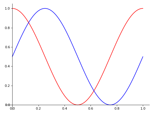
如果有多个绘图,则相同的可选参数将应用于在同一画布中绘制的所有绘图。如果要单独设置这些选项,可以为返回的
Plot对象并设置它。例如,当您指定
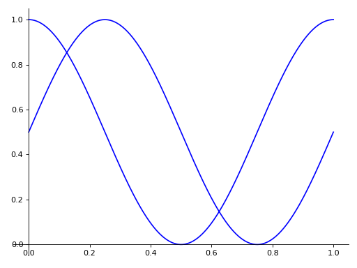
line_color一旦,它将同时适用于两个系列。>>> from sympy import pi >>> expr1 = (u, cos(2*pi*u)/2 + 1/2) >>> expr2 = (u, sin(2*pi*u)/2 + 1/2) >>> p = plot_parametric(expr1, expr2, (u, 0, 1), line_color='blue')
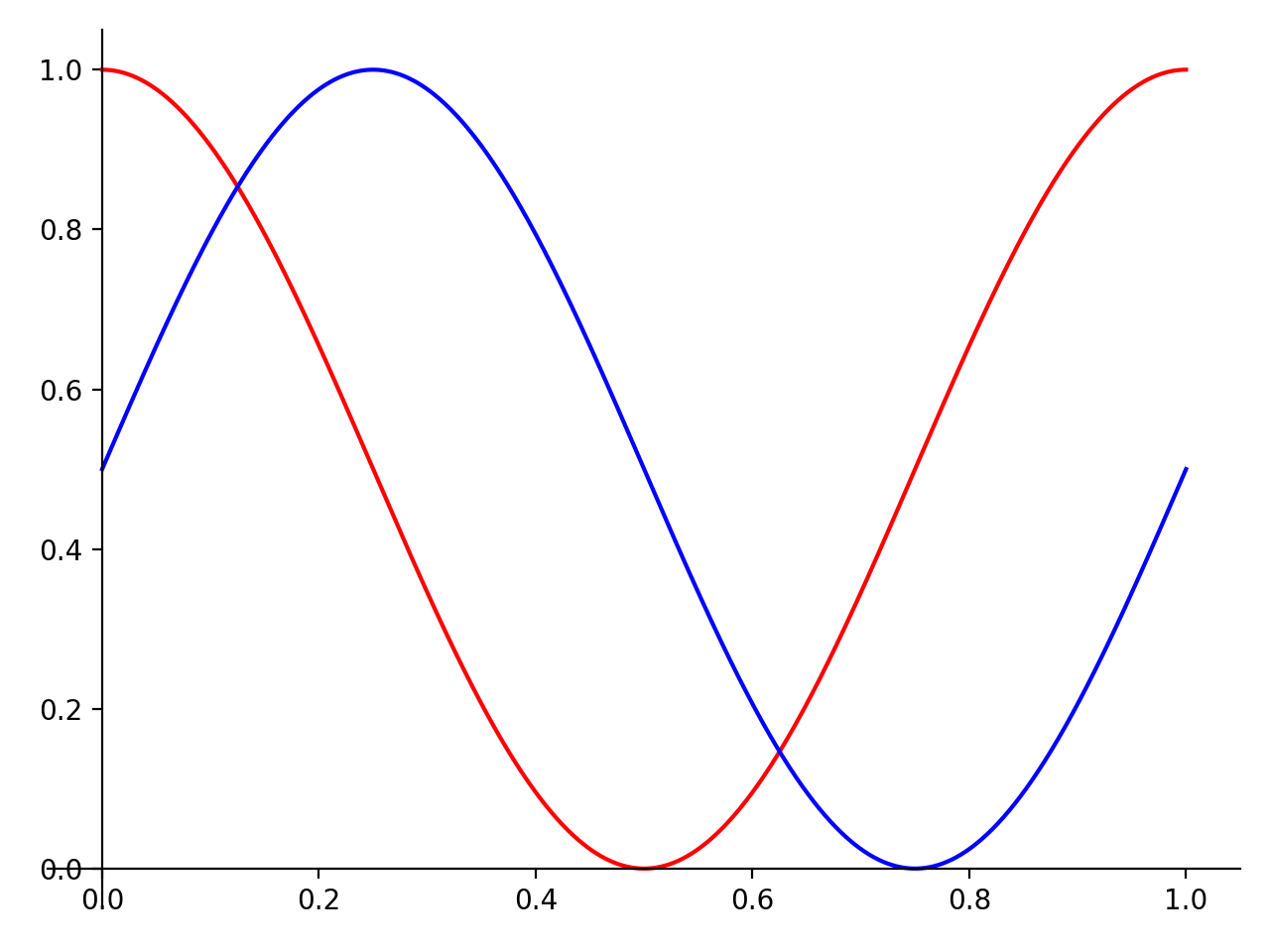
如果要为特定系列指定线条颜色,则应为每个项目编制索引并手动应用该属性。
>>> p[0].line_color = 'red'
>>> p.show()

- sympy.plotting.plot.plot3d(*args, show=True, **kwargs)[源代码]#
打印三维曲面打印。
使用
单一地块
plot3d(expr, range_x, range_y, **kwargs)如果未指定范围,则使用默认范围(-10,10)。
同一范围的多重绘图。
plot3d(expr1, expr2, range_x, range_y, **kwargs)如果未指定范围,则使用默认范围(-10,10)。
具有不同范围的多个绘图。
plot3d((expr1, range_x, range_y), (expr2, range_x, range_y), ..., **kwargs)必须为每个表达式指定范围。
如果实施更先进的默认范围检测算法,默认范围将来可能会发生变化。
争论
expr : Expression representing the function along x.
- range_x(
Symbol, float, float) A 3-tuple denoting the range of the x variable, e.g. (x, 0, 5).
- range_y(
Symbol, float, float) A 3-tuple denoting the range of the y variable, e.g. (y, 0, 5).
关键字参数
的参数
SurfaceOver2DRangeSeries班级:- n1利息
The x range is sampled uniformly at
n1of points. This keyword argument replacesnb_of_points_x, which should be considered deprecated.- n2利息
The y range is sampled uniformly at
n2of points. This keyword argument replacesnb_of_points_y, which should be considered deprecated.
美学:
- surface_colorFunction which returns a float
Specifies the color for the surface of the plot. See
Plotfor more details.
如果有多个绘图,则对所有绘图应用相同的系列参数。如果要单独设置这些选项,可以为返回的
Plot对象并设置它。的参数
Plot班级:- titleSTR
Title of the plot.
- 大小(浮动,浮动)可选
以英寸为单位的形式(宽度、高度)的元组,用于指定整个图形的大小。默认值设置为
None,这意味着大小将由默认后端设置。
实例
>>> from sympy import symbols
>>> from sympy.plotting import plot3d
>>> x, y = symbols('x y')
单一地块
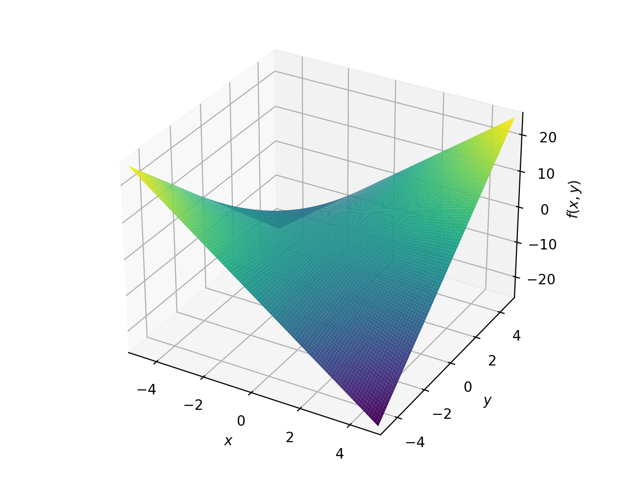
>>> plot3d(x*y, (x, -5, 5), (y, -5, 5))
Plot object containing:
[0]: cartesian surface: x*y for x over (-5.0, 5.0) and y over (-5.0, 5.0)

具有相同范围的多个绘图
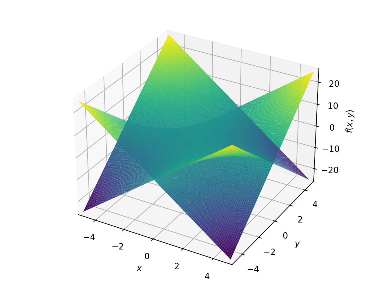
>>> plot3d(x*y, -x*y, (x, -5, 5), (y, -5, 5))
Plot object containing:
[0]: cartesian surface: x*y for x over (-5.0, 5.0) and y over (-5.0, 5.0)
[1]: cartesian surface: -x*y for x over (-5.0, 5.0) and y over (-5.0, 5.0)

具有不同范围的多个绘图。
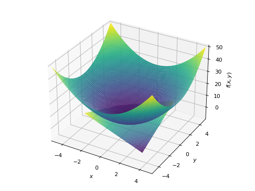
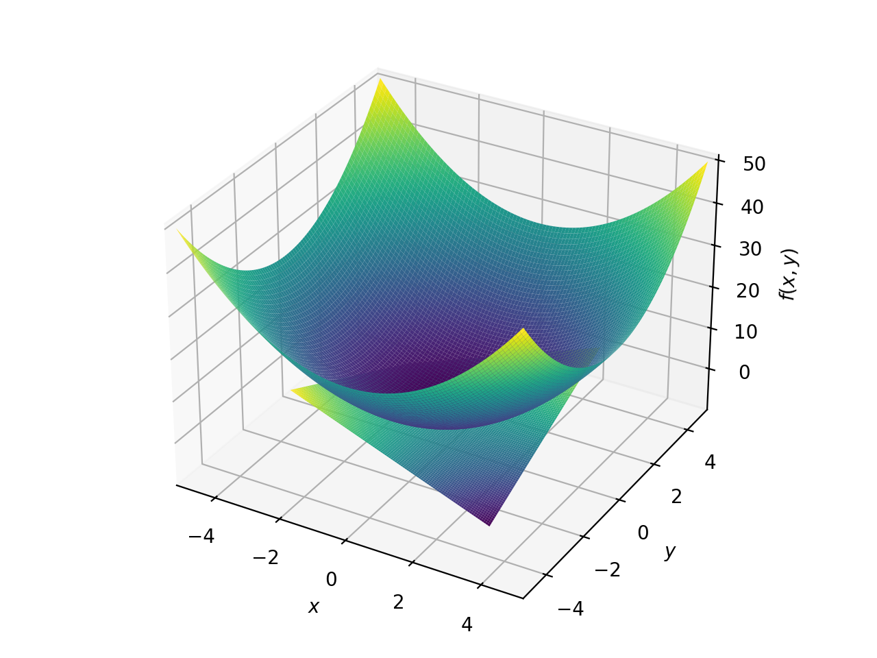
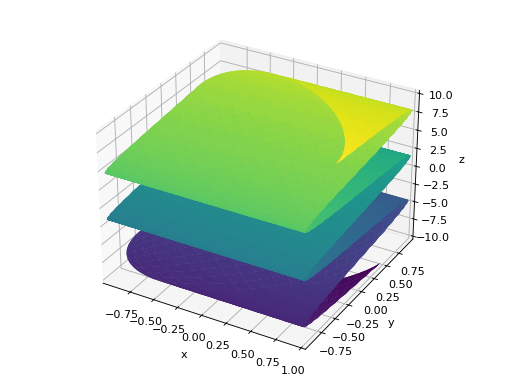
>>> plot3d((x**2 + y**2, (x, -5, 5), (y, -5, 5)),
...     (x*y, (x, -3, 3), (y, -3, 3)))
Plot object containing:
[0]: cartesian surface: x**2 + y**2 for x over (-5.0, 5.0) and y over (-5.0, 5.0)
[1]: cartesian surface: x*y for x over (-3.0, 3.0) and y over (-3.0, 3.0)

- range_x(
- sympy.plotting.plot.plot3d_parametric_line(*args, show=True, **kwargs)[源代码]#
打印三维参数化直线打印。
使用
单一地块:
plot3d_parametric_line(expr_x, expr_y, expr_z, range, **kwargs)如果未指定范围,则使用默认范围(-10,10)。
多个绘图。
plot3d_parametric_line((expr_x, expr_y, expr_z, range), ..., **kwargs)必须为每个表达式指定范围。
如果实施更先进的默认范围检测算法,默认范围将来可能会发生变化。
争论
expr_x : Expression representing the function along x.
expr_y : Expression representing the function along y.
expr_z : Expression representing the function along z.
- range(
Symbol, float, float) A 3-tuple denoting the range of the parameter variable, e.g., (u, 0, 5).
关键字参数
的参数
Parametric3DLineSeries班级。- N号利息
The range is uniformly sampled at
nnumber of points. This keyword argument replacesnb_of_points, which should be considered deprecated.
美学:
- line_colorstring, or float, or function, optional
Specifies the color for the plot. See
Plotto see how to set color for the plots. Note that by settingline_color, it would be applied simultaneously to all the series.- labelSTR
绘图的标签。它将在调用时使用
legend=True在绘图中用给定的标签来表示函数。
如果有多个绘图,则对所有绘图应用相同的系列参数。如果要单独设置这些选项,可以为返回的
Plot对象并设置它。的参数
Plot班级。- titleSTR
Title of the plot.
- 大小(浮动,浮动)可选
以英寸为单位的形式(宽度、高度)的元组,用于指定整个图形的大小。默认值设置为
None,这意味着大小将由默认后端设置。
实例
>>> from sympy import symbols, cos, sin
>>> from sympy.plotting import plot3d_parametric_line
>>> u = symbols('u')
单一地块。
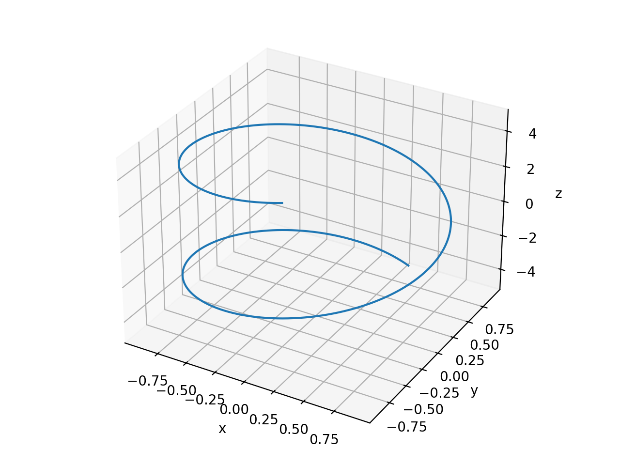
>>> plot3d_parametric_line(cos(u), sin(u), u, (u, -5, 5))
Plot object containing:
[0]: 3D parametric cartesian line: (cos(u), sin(u), u) for u over (-5.0, 5.0)

多个绘图。
>>> plot3d_parametric_line((cos(u), sin(u), u, (u, -5, 5)),
...     (sin(u), u**2, u, (u, -5, 5)))
Plot object containing:
[0]: 3D parametric cartesian line: (cos(u), sin(u), u) for u over (-5.0, 5.0)
[1]: 3D parametric cartesian line: (sin(u), u**2, u) for u over (-5.0, 5.0)
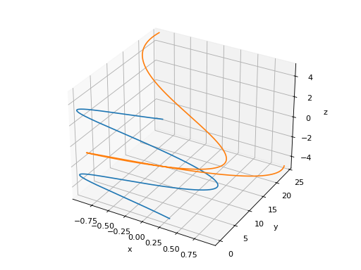
- range(
- sympy.plotting.plot.plot3d_parametric_surface(*args, show=True, **kwargs)[源代码]#
打印三维参数化曲面打印。
解释
单一地块。
plot3d_parametric_surface(expr_x, expr_y, expr_z, range_u, range_v, **kwargs)如果未指定范围,则使用默认范围(-10,10)。
多个绘图。
plot3d_parametric_surface((expr_x, expr_y, expr_z, range_u, range_v), ..., **kwargs)必须为每个表达式指定范围。
如果实施更先进的默认范围检测算法,默认范围将来可能会发生变化。
争论
expr_x : Expression representing the function along
x.expr_y : Expression representing the function along
y.expr_z : Expression representing the function along
z.- range_u(
Symbol, float, float) A 3-tuple denoting the range of the u variable, e.g. (u, 0, 5).
- range_v(
Symbol, float, float) A 3-tuple denoting the range of the v variable, e.g. (v, 0, 5).
关键字参数
的参数
ParametricSurfaceSeries班级:- n1利息
The
urange is sampled uniformly atn1of points. This keyword argument replacesnb_of_points_u, which should be considered deprecated.- n2利息
The
vrange is sampled uniformly atn2of points. This keyword argument replacesnb_of_points_v, which should be considered deprecated.
美学:
- surface_colorFunction which returns a float
Specifies the color for the surface of the plot. See
Plotfor more details.
如果有多个绘图,则对所有绘图应用相同的系列参数。如果要单独设置这些选项,可以为返回的
Plot对象并设置它。的参数
Plot班级:- titleSTR
Title of the plot.
- 大小(浮动,浮动)可选
以英寸为单位的形式(宽度、高度)的元组,用于指定整个图形的大小。默认值设置为
None,这意味着大小将由默认后端设置。
实例
>>> from sympy import symbols, cos, sin
>>> from sympy.plotting import plot3d_parametric_surface
>>> u, v = symbols('u v')
单一地块。
>>> plot3d_parametric_surface(cos(u + v), sin(u - v), u - v,
...     (u, -5, 5), (v, -5, 5))
Plot object containing:
[0]: parametric cartesian surface: (cos(u + v), sin(u - v), u - v) for u over (-5.0, 5.0) and v over (-5.0, 5.0)
- range_u(
- sympy.plotting.plot_implicit.plot_implicit(expr, x_var=None, y_var=None, adaptive=True, depth=0, n=300, line_color='blue', show=True, **kwargs)[源代码]#
绘制隐式方程/不等式的绘图函数。
争论
expr : The equation / inequality that is to be plotted.
x_var (optional) : symbol to plot on x-axis or tuple giving symbol and range as
(symbol, xmin, xmax)y_var (optional) : symbol to plot on y-axis or tuple giving symbol and range as
(symbol, ymin, ymax)
如果既不
x_var也不y_var则表达式中的自由符号将按排序顺序分配。还可以使用以下关键字参数:
adaptive布尔值。默认值设置为True。一定是的如果要使用网格栅格,请设置为False。
depth整数。自适应网格网格的递归深度。默认值为0。取值范围为(0,4)。
ninteger. The number of points if adaptive mesh grid is notused. Default value is 300. This keyword argument replaces
points, which should be considered deprecated.
show布尔值。默认值为True。如果设置为False,则绘图将不显示。看到了吗
Plot更多信息。
title字符串。情节的标题。xlabel字符串。x轴的标签ylabel字符串。y轴的标签
美学选项:
line_color:浮点或字符串。指定打印的颜色。见
Plot查看如何为绘图设置颜色。默认值为“蓝色”
默认情况下,plot_implicit使用区间算术来绘制函数。如果无法使用区间算术绘制表达式,则默认为使用固定点数的网格网格生成轮廓。通过将“自适应”设置为False,可以强制plot峎隐式使用网格网格。网格网格法在采用区间算法进行自适应绘图时是有效的,不能以较小的线宽绘制。
实例
绘图表达式:
>>> from sympy import plot_implicit, symbols, Eq, And
>>> x, y = symbols('x y')
表达式中的符号没有任何范围:
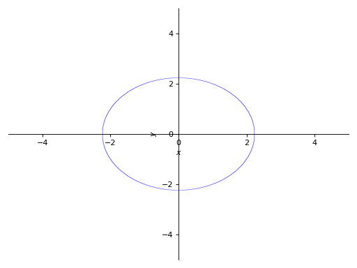
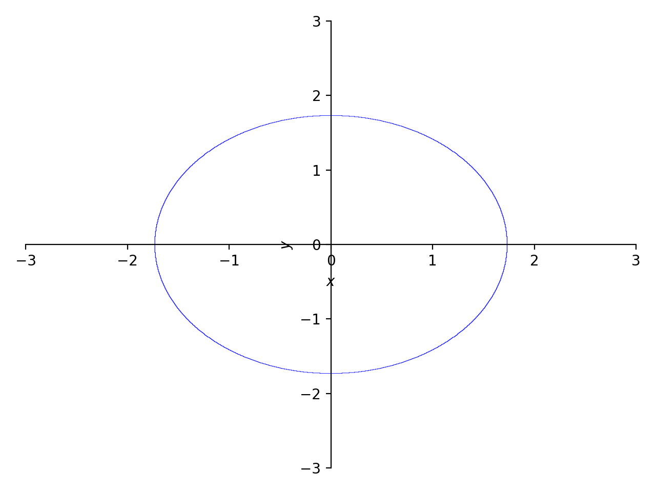
>>> p1 = plot_implicit(Eq(x**2 + y**2, 5))

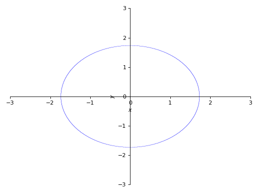
符号范围:
>>> p2 = plot_implicit(
...     Eq(x**2 + y**2, 3), (x, -3, 3), (y, -3, 3))

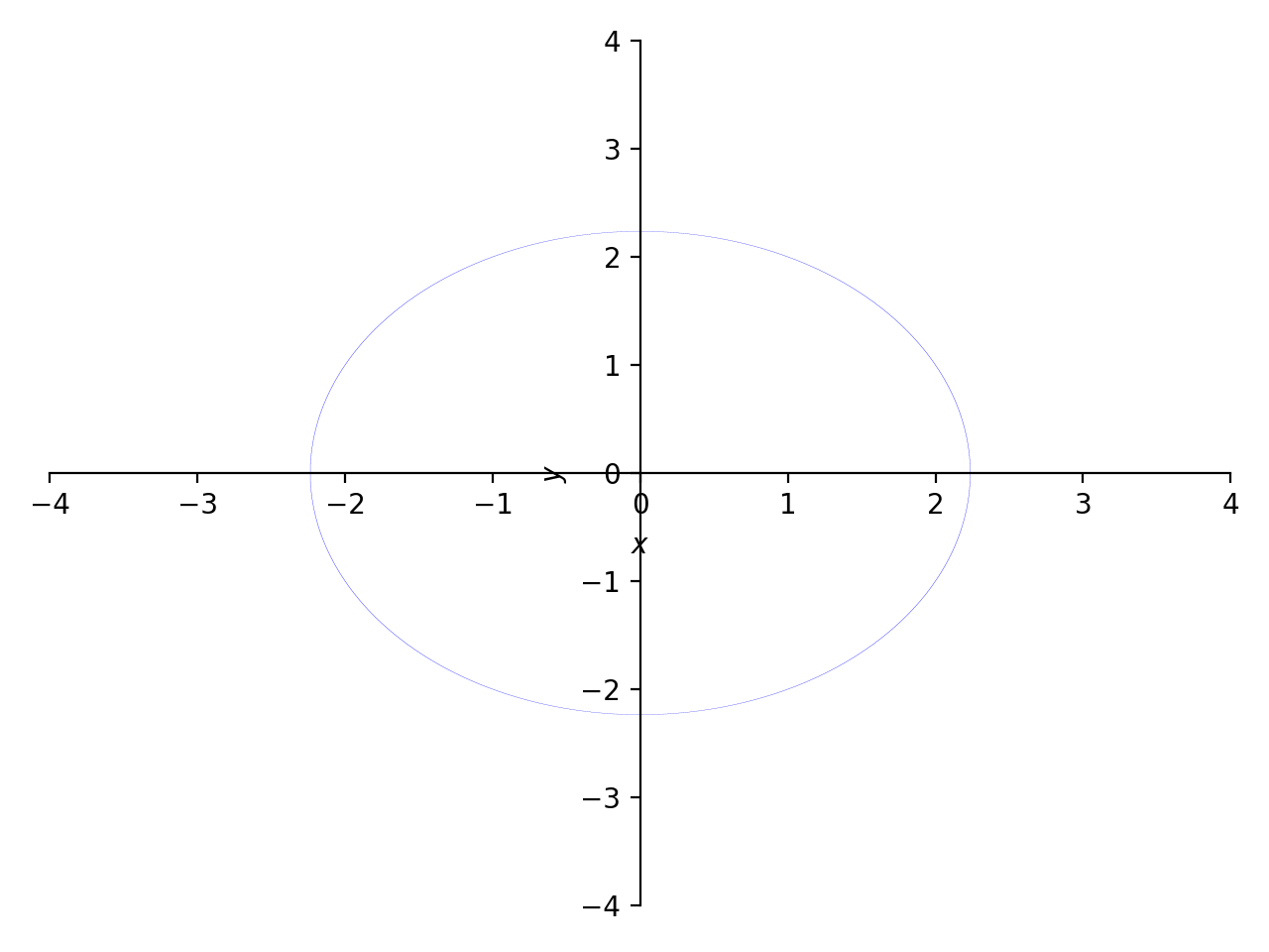
以递归深度为参数:
>>> p3 = plot_implicit(
...     Eq(x**2 + y**2, 5), (x, -4, 4), (y, -4, 4), depth = 2)
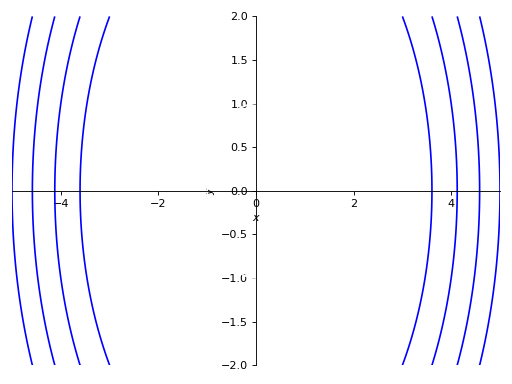
使用网格网格而不使用自适应网格:
>>> p4 = plot_implicit(
...     Eq(x**2 + y**2, 5), (x, -5, 5), (y, -2, 2),
...     adaptive=False)

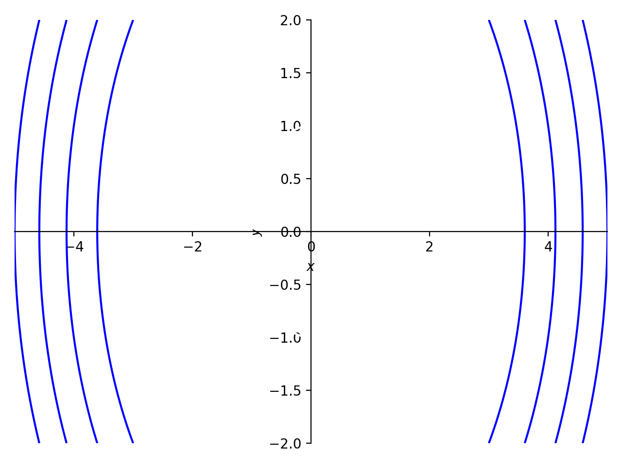
使用网格网格而不使用指定点数的自适应网格:
>>> p5 = plot_implicit(
...     Eq(x**2 + y**2, 5), (x, -5, 5), (y, -2, 2),
...     adaptive=False, n=400)

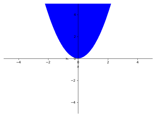
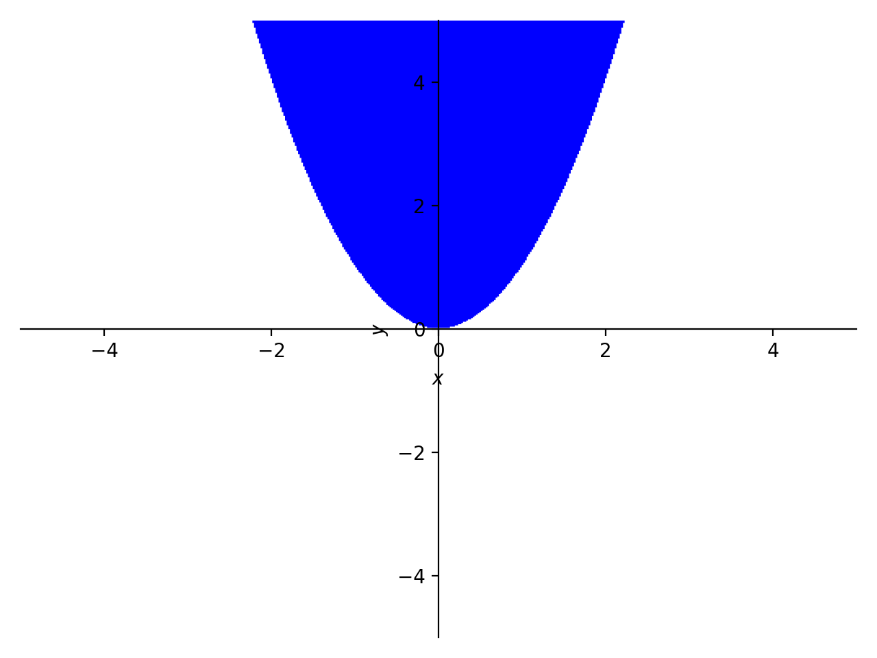
绘图区域:
>>> p6 = plot_implicit(y > x**2)

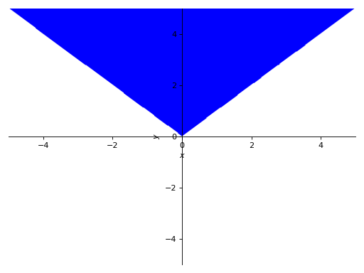
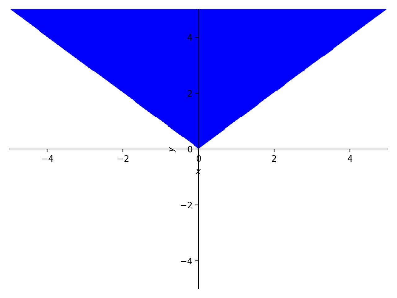
使用布尔连接绘制:
>>> p7 = plot_implicit(And(y > x, y > -x))

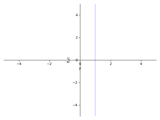
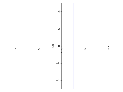
当用单个变量(例如y-1)绘制表达式时,请显式指定x或y变量:
>>> p8 = plot_implicit(y - 1, y_var=y)
>>> p9 = plot_implicit(x - 1, x_var=x)
PlotGrid类#
- class sympy.plotting.plot.PlotGrid(nrows, ncolumns, *args, show=True, size=None, **kwargs)[源代码]#
This class helps to plot subplots from already created SymPy plots in a single figure.
实例
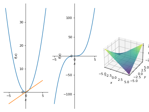
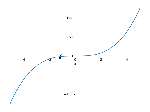
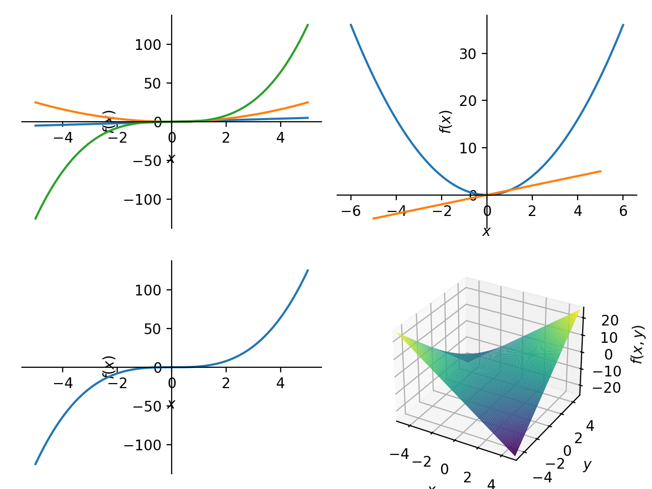
>>> from sympy import symbols
>>> from sympy.plotting import plot, plot3d, PlotGrid
>>> x, y = symbols('x, y')
>>> p1 = plot(x, x**2, x**3, (x, -5, 5))
>>> p2 = plot((x**2, (x, -6, 6)), (x, (x, -5, 5)))
>>> p3 = plot(x**3, (x, -5, 5))
>>> p4 = plot3d(x*y, (x, -5, 5), (y, -5, 5))


在一条直线上垂直打印:
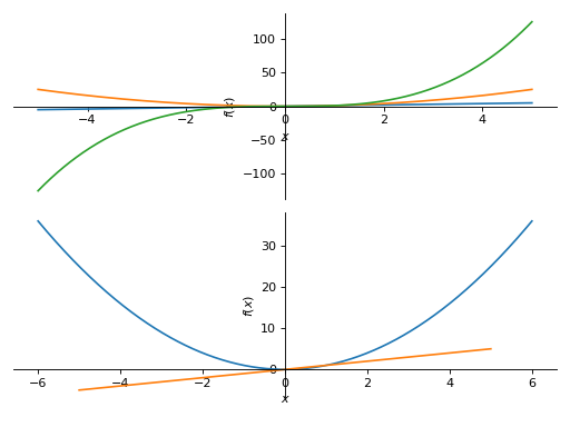
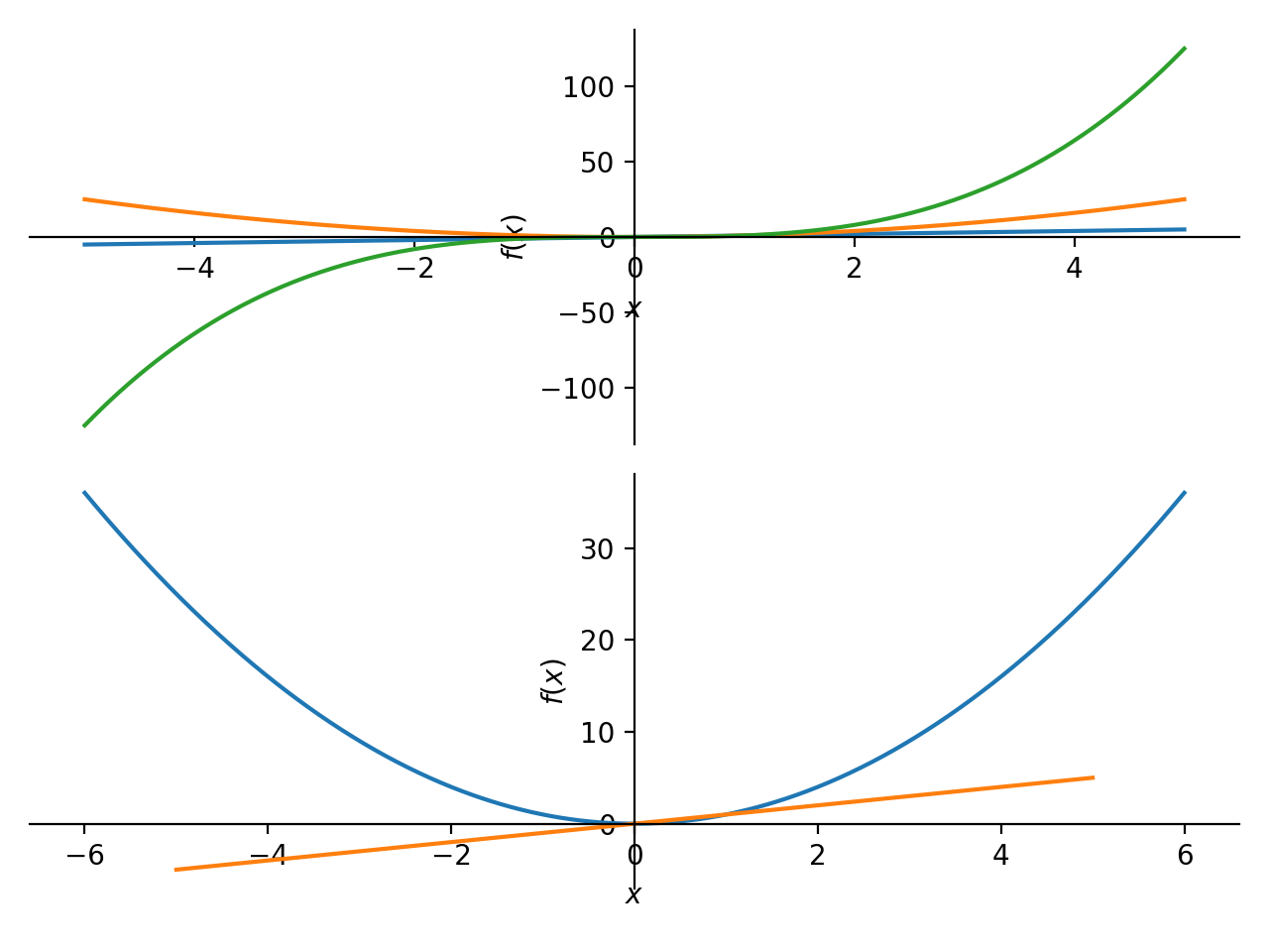
>>> PlotGrid(2, 1, p1, p2)
PlotGrid object containing:
Plot[0]:Plot object containing:
[0]: cartesian line: x for x over (-5.0, 5.0)
[1]: cartesian line: x**2 for x over (-5.0, 5.0)
[2]: cartesian line: x**3 for x over (-5.0, 5.0)
Plot[1]:Plot object containing:
[0]: cartesian line: x**2 for x over (-6.0, 6.0)
[1]: cartesian line: x for x over (-5.0, 5.0)

在单行中水平绘制:
>>> PlotGrid(1, 3, p2, p3, p4)
PlotGrid object containing:
Plot[0]:Plot object containing:
[0]: cartesian line: x**2 for x over (-6.0, 6.0)
[1]: cartesian line: x for x over (-5.0, 5.0)
Plot[1]:Plot object containing:
[0]: cartesian line: x**3 for x over (-5.0, 5.0)
Plot[2]:Plot object containing:
[0]: cartesian surface: x*y for x over (-5.0, 5.0) and y over (-5.0, 5.0)
以网格形式打印:
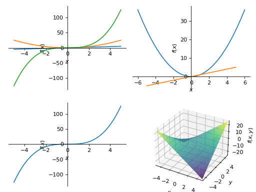
>>> PlotGrid(2, 2, p1, p2, p3, p4)
PlotGrid object containing:
Plot[0]:Plot object containing:
[0]: cartesian line: x for x over (-5.0, 5.0)
[1]: cartesian line: x**2 for x over (-5.0, 5.0)
[2]: cartesian line: x**3 for x over (-5.0, 5.0)
Plot[1]:Plot object containing:
[0]: cartesian line: x**2 for x over (-6.0, 6.0)
[1]: cartesian line: x for x over (-5.0, 5.0)
Plot[2]:Plot object containing:
[0]: cartesian line: x**3 for x over (-5.0, 5.0)
Plot[3]:Plot object containing:
[0]: cartesian surface: x*y for x over (-5.0, 5.0) and y over (-5.0, 5.0)

系列课程#
- class sympy.plotting.series.BaseSeries(*args, **kwargs)[源代码]#
包含要打印的内容的数据对象的基类。
笔记
The backend should check if it supports the data series that is given. (e.g. TextBackend supports only LineOver1DRangeSeries). It is the backend responsibility to know how to use the class of data series that is given.
Some data series classes are grouped (using a class attribute like is_2Dline) according to the api they present (based only on convention). The backend is not obliged to use that api (e.g. LineOver1DRangeSeries belongs to the is_2Dline group and presents the get_points method, but the TextBackend does not use the get_points method).
BaseSeries
- eval_color_func(*args)[源代码]#
Evaluate the color function.
- 参数:
args :元组
Arguments to be passed to the coloring function. Can be coordinates or parameters or both.
笔记
The backend will request the data series to generate the numerical data. Depending on the data series, either the data series itself or the backend will eventually execute this function to generate the appropriate coloring value.
- property expr#
Return the expression (or expressions) of the series.
- get_data()[源代码]#
Compute and returns the numerical data.
The number of parameters returned by this method depends on the specific instance. If
sis the series, make sure to readhelp(s.get_data)to understand what it returns.
- get_label(use_latex=False, wrapper='$%s$')[源代码]#
Return the label to be used to display the expression.
- 参数:
use_latex : bool
If False, the string representation of the expression is returned. If True, the latex representation is returned.
wrapper : str
The backend might need the latex representation to be wrapped by some characters. Default to
"$%s$".- 返回:
label : str
- property n#
Returns a list [n1, n2, n3] of numbers of discratization points.
- property params#
Get or set the current parameters dictionary.
- 参数:
p : dict
key: symbol associated to the parameter
val: the numeric value
- class sympy.plotting.series.Line2DBaseSeries(**kwargs)[源代码]#
二维线的基类。
添加label、steps和only-integers选项
制造是真的吗
定义get_段和get_color_数组
- get_data()[源代码]#
Return coordinates for plotting the line.
- 返回:
x: np.ndarray
x-coordinates
y: np.ndarray
y-coordinates
z: np.ndarray (optional)
z-coordinates in case of Parametric3DLineSeries, Parametric3DLineInteractiveSeries
param : np.ndarray (optional)
The parameter in case of Parametric2DLineSeries, Parametric3DLineSeries or AbsArgLineSeries (and their corresponding interactive series).
- class sympy.plotting.series.LineOver1DRangeSeries(expr, var_start_end, label='', **kwargs)[源代码]#
在一定范围内由一个辛表达式组成的线的表示。
- get_points()[源代码]#
Return lists of coordinates for plotting. Depending on the
adaptiveoption, this function will either use an adaptive algorithm or it will uniformly sample the expression over the provided range.This function is available for back-compatibility purposes. Consider using
get_data()instead.- 返回:
x : list
List of x-coordinates
- Y列表
List of y-coordinates
- class sympy.plotting.series.Parametric2DLineSeries(expr_x, expr_y, var_start_end, label='', **kwargs)[源代码]#
Representation for a line consisting of two parametric SymPy expressions over a range.
- class sympy.plotting.series.Parametric3DLineSeries(expr_x, expr_y, expr_z, var_start_end, label='', **kwargs)[源代码]#
Representation for a 3D line consisting of three parametric SymPy expressions and a range.
- class sympy.plotting.series.SurfaceOver2DRangeSeries(expr, var_start_end_x, var_start_end_y, label='', **kwargs)[源代码]#
Representation for a 3D surface consisting of a SymPy expression and 2D range.
- class sympy.plotting.series.ParametricSurfaceSeries(expr_x, expr_y, expr_z, var_start_end_u, var_start_end_v, label='', **kwargs)[源代码]#
Representation for a 3D surface consisting of three parametric SymPy expressions and a range.
- class sympy.plotting.series.ImplicitSeries(expr, var_start_end_x, var_start_end_y, label='', **kwargs)[源代码]#
Representation for 2D Implicit plot.
- get_data()[源代码]#
Returns numerical data.
- 返回:
If the series is evaluated with the \(adaptive=True\) it returns:
interval_list : list
List of bounding rectangular intervals to be postprocessed and eventually used with Matplotlib's
fillcommand.dummy : str
A string containing
"fill".Otherwise, it returns 2D numpy arrays to be used with Matplotlib's
contourorcontourfcommands:x_array : np.ndarray
y_array : np.ndarray
z_array : np.ndarray
plot_type : str
A string specifying which plot command to use,
"contour"or"contourf".
- get_label(use_latex=False, wrapper='$%s$')[源代码]#
Return the label to be used to display the expression.
- 参数:
use_latex : bool
If False, the string representation of the expression is returned. If True, the latex representation is returned.
wrapper : str
The backend might need the latex representation to be wrapped by some characters. Default to
"$%s$".- 返回:
label : str
后端#
- class sympy.plotting.plot.MatplotlibBackend(*series, **kwargs)[源代码]#
此类实现了将Matplotlib与SymPy打印函数一起使用的功能。
- static get_segments(x, y, z=None)[源代码]#
Convert two list of coordinates to a list of segments to be used with Matplotlib's
LineCollection.- 参数:
x : list
List of x-coordinates
- Y列表
List of y-coordinates
- Z列表
List of z-coordinates for a 3D line.
Pyglet绘图#
这是使用pyglet的旧打印模块的文档。此模块有一些局限性,不再积极开发。另一种方法是查看新的绘图模块。
The pyglet plotting module can do nice 2D and 3D plots that can be controlled by console commands as well as keyboard and mouse, with the only dependency being pyglet.
以下是最简单的用法:
>>> from sympy import var
>>> from sympy.plotting.pygletplot import PygletPlot as Plot
>>> var('x y z')
>>> Plot(x*y**3-y*x**3)
To see lots of plotting examples, see examples/pyglet_plotting.py and try running
it in interactive mode (python -i plotting.py):
$ python -i examples/pyglet_plotting.py
和类型,例如 example(7) 或 example(11) .
也见 Plotting Module 截图的wiki页面。
绘图窗口控件#
照相机 |
钥匙 |
|---|---|
灵敏度调整器 |
SHIFT |
变焦 |
R和F,上下翻页,Numpad+和- |
旋转视图X、Y轴 |
箭头键,A、S、D、W、Numpad 4、6、8、2 |
旋转视图Z轴 |
Q和E,Numpad 7和9 |
旋转坐标Z轴 |
Z和C,Numpad 1和3 |
视图XY |
一层楼 |
视图XZ |
地上二层 |
查看YZ |
三层 |
透视图 |
4层 |
重置 |
十、 纽帕德5 |
轴线 |
钥匙 |
|---|---|
切换可见 |
5楼 |
切换颜色 |
F6层 |
窗口 |
钥匙 |
|---|---|
关闭 |
ESCAPE |
截图 |
8楼 |
鼠标可以通过拖动鼠标左键、中键和右键来旋转、缩放和平移。
坐标模式#
Plot 支持多种曲线坐标模式,它们对每个绘图函数都是独立的。可以使用名为“mode”的参数显式指定坐标模式,但可以为笛卡尔或参数化绘图自动确定坐标模式,因此只能为极轴模式、柱面模式和球形模式指定坐标模式。
明确地, Plot(function arguments) 和 Plot.__setitem__(i, function arguments) (使用数组索引语法访问 Plot 如果提供一个函数,则将参数解释为笛卡尔图;如果提供两个或三个函数,则将参数解释为参数图。类似地,参数将被解释为使用一个变量的曲线,如果使用两个变量,则解释为曲面。
支持的变量数模式:
1(曲线):参数化、笛卡尔、极坐标
2(曲面):参数化、笛卡尔、圆柱形、球形
>>> Plot(1, 'mode=spherical; color=zfade4')
Note that function parameters are given as option strings of the form
"key1=value1; key2 = value2" (spaces are truncated). Keyword arguments given
directly to plot apply to the plot itself.
指定变量的间隔#
可变间隔的基本格式是 [变量、最小值、最大值、步数] . 但是,语法非常灵活,未指定的参数取自当前坐标模式的默认值:
>>> Plot(x**2) # implies [x,-5,5,100]
>>> Plot(x**2, [], []) # [x,-1,1,40], [y,-1,1,40]
>>> Plot(x**2-y**2, [100], [100]) # [x,-1,1,100], [y,-1,1,100]
>>> Plot(x**2, [x,-13,13,100])
>>> Plot(x**2, [-13,13]) # [x,-13,13,100]
>>> Plot(x**2, [x,-13,13]) # [x,-13,13,100]
>>> Plot(1*x, [], [x], 'mode=cylindrical') # [unbound_theta,0,2*Pi,40], [x,-1,1,20]
使用交互界面#
>>> p = Plot(visible=False)
>>> f = x**2
>>> p[1] = f
>>> p[2] = f.diff(x)
>>> p[3] = f.diff(x).diff(x)
>>> p
[1]: x**2, 'mode=cartesian'
[2]: 2*x, 'mode=cartesian'
[3]: 2, 'mode=cartesian'
>>> p.show()
>>> p.clear()
>>> p
<blank plot>
>>> p[1] =  x**2+y**2
>>> p[1].style = 'solid'
>>> p[2] = -x**2-y**2
>>> p[2].style = 'wireframe'
>>> p[1].color = z, (0.4,0.4,0.9), (0.9,0.4,0.4)
>>> p[1].style = 'both'
>>> p[2].style = 'both'
>>> p.close()
使用自定义颜色函数#
以下代码将绘制鞍座并根据其渐变的大小对其进行着色:
>>> fz = x**2-y**2
>>> Fx, Fy, Fz = fz.diff(x), fz.diff(y), 0
>>> p[1] = fz, 'style=solid'
>>> p[1].color = (Fx**2 + Fy**2 + Fz**2)**(0.5)
着色算法的工作原理如下:
计算曲线或曲面上的颜色函数。
求出每个分量的最小值和最大值。
将每个组件缩放到颜色渐变。
When not specified explicitly, the default color gradient is \(f(0.0)=(0.4,0.4,0.4) \rightarrow f(1.0)=(0.9,0.9,0.9)\). In our case, everything is gray-scale because we have applied the default color gradient uniformly for each color component. When defining a color scheme in this way, you might want to supply a color gradient as well:
>>> p[1].color = (Fx**2 + Fy**2 + Fz**2)**(0.5), (0.1,0.1,0.9), (0.9,0.1,0.1)
这里有四个步骤的颜色渐变:
>>> gradient = [ 0.0, (0.1,0.1,0.9), 0.3, (0.1,0.9,0.1),
...              0.7, (0.9,0.9,0.1), 1.0, (1.0,0.0,0.0) ]
>>> p[1].color = (Fx**2 + Fy**2 + Fz**2)**(0.5), gradient
指定颜色方案的另一种方法是为每个组件r、g、b提供单独的函数。使用此语法,默认颜色方案定义如下:
>>> p[1].color = z,y,x, (0.4,0.4,0.4), (0.9,0.9,0.9)
这将映射z->红色、y->绿色和x->蓝色。在某些情况下,您可能更喜欢使用以下替代语法:
>>> p[1].color = z,(0.4,0.9), y,(0.4,0.9), x,(0.4,0.9)
您仍然可以将多步渐变与三个函数配色方案一起使用。
绘制几何实体#
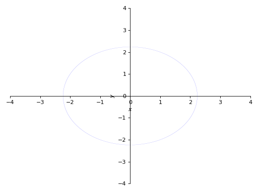
The plotting module is capable of plotting some 2D geometric entities like line, circle and ellipse. The following example plots a circle centred at origin and of radius 2 units.
>>> from sympy import *
>>> x,y = symbols('x y')
>>> plot_implicit(Eq(x**2+y**2, 4))
Similarly, plot_implicit() may be used to plot any 2-D geometric structure from
its implicit equation.
Plotting polygons (Polygon, RegularPolygon, Triangle) are not supported directly.
用ASCII图形绘制#
- sympy.plotting.textplot.textplot(expr, a, b, W=55, H=21)[源代码]#
打印一张完整的ASCII艺术图,其中包含一个符号,例如x或其他符号 [a, b] .
实例
>>> from sympy import Symbol, sin
>>> from sympy.plotting import textplot
>>> t = Symbol('t')
>>> textplot(sin(t)*t, 0, 15)
 14 |                                                  ...
    |                                                     .
    |                                                 .
    |                                                      .
    |                                                .
    |                            ...
    |                           /   .               .
    |                          /
    |                         /      .
    |                        .        .            .
1.5 |----.......--------------------------------------------
    |....       \           .          .
    |            \         /                      .
    |             ..      /             .
    |               \    /                       .
    |                ....
    |                                    .
    |                                     .     .
    |
    |                                      .   .
-11 |_______________________________________________________
     0                          7.5                        15