梁(Docstrings)#
该模块可用于求解具有奇异函数的二维梁弯曲问题。
- class sympy.physics.continuum_mechanics.beam.Beam(length, elastic_modulus, second_moment, area=A, variable=x, base_char='C')[源代码]#
梁是一种主要通过抗弯来承受荷载的结构构件。梁的特征在于其横截面轮廓(面积二阶矩)、长度和材料。
备注
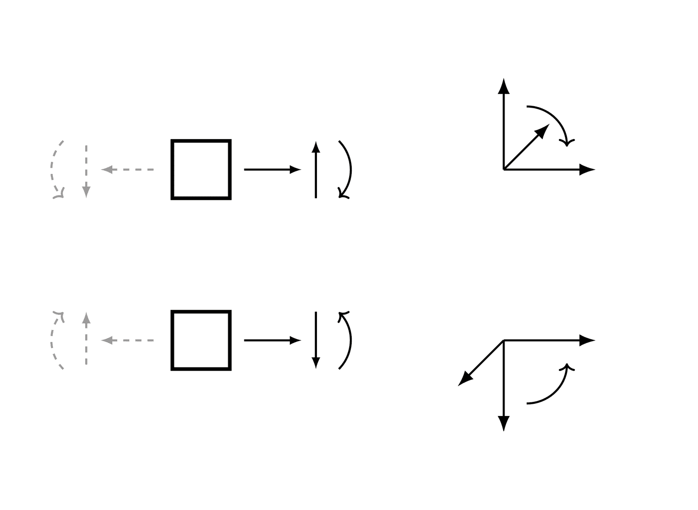
A consistent sign convention must be used while solving a beam bending problem; the results will automatically follow the chosen sign convention. However, the chosen sign convention must respect the rule that, on the positive side of beam's axis (in respect to current section), a loading force giving positive shear yields a negative moment, as below (the curved arrow shows the positive moment and rotation):
实例
有一根4米长的横梁。从梁的一半到梁端施加6 N/m的恒定分布荷载。在梁的下方有两个简支,一个在梁的起点,另一个在梁的终点。梁端的挠度受到限制。
使用向下力为正的符号约定。
>>> from sympy.physics.continuum_mechanics.beam import Beam
>>> from sympy import symbols, Piecewise
>>> E, I = symbols('E, I')
>>> R1, R2 = symbols('R1, R2')
>>> b = Beam(4, E, I)
>>> b.apply_load(R1, 0, -1)
>>> b.apply_load(6, 2, 0)
>>> b.apply_load(R2, 4, -1)
>>> b.bc_deflection = [(0, 0), (4, 0)]
>>> b.boundary_conditions
{'deflection': [(0, 0), (4, 0)], 'slope': []}
>>> b.load
R1*SingularityFunction(x, 0, -1) + R2*SingularityFunction(x, 4, -1) + 6*SingularityFunction(x, 2, 0)
>>> b.solve_for_reaction_loads(R1, R2)
>>> b.load
-3*SingularityFunction(x, 0, -1) + 6*SingularityFunction(x, 2, 0) - 9*SingularityFunction(x, 4, -1)
>>> b.shear_force()
3*SingularityFunction(x, 0, 0) - 6*SingularityFunction(x, 2, 1) + 9*SingularityFunction(x, 4, 0)
>>> b.bending_moment()
3*SingularityFunction(x, 0, 1) - 3*SingularityFunction(x, 2, 2) + 9*SingularityFunction(x, 4, 1)
>>> b.slope()
(-3*SingularityFunction(x, 0, 2)/2 + SingularityFunction(x, 2, 3) - 9*SingularityFunction(x, 4, 2)/2 + 7)/(E*I)
>>> b.deflection()
(7*x - SingularityFunction(x, 0, 3)/2 + SingularityFunction(x, 2, 4)/4 - 3*SingularityFunction(x, 4, 3)/2)/(E*I)
>>> b.deflection().rewrite(Piecewise)
(7*x - Piecewise((x**3, x >= 0), (0, True))/2
     - 3*Piecewise(((x - 4)**3, x >= 4), (0, True))/2
     + Piecewise(((x - 2)**4, x >= 2), (0, True))/4)/(E*I)
Calculate the support reactions for a fully symbolic beam of length L. There are two simple supports below the beam, one at the starting point and another at the ending point of the beam. The deflection of the beam at the end is restricted. The beam is loaded with:
a downward point load P1 applied at L/4
an upward point load P2 applied at L/8
a counterclockwise moment M1 applied at L/2
a clockwise moment M2 applied at 3*L/4
a distributed constant load q1, applied downward, starting from L/2 up to 3*L/4
a distributed constant load q2, applied upward, starting from 3*L/4 up to L
No assumptions are needed for symbolic loads. However, defining a positive length will help the algorithm to compute the solution.
>>> E, I = symbols('E, I')
>>> L = symbols("L", positive=True)
>>> P1, P2, M1, M2, q1, q2 = symbols("P1, P2, M1, M2, q1, q2")
>>> R1, R2 = symbols('R1, R2')
>>> b = Beam(L, E, I)
>>> b.apply_load(R1, 0, -1)
>>> b.apply_load(R2, L, -1)
>>> b.apply_load(P1, L/4, -1)
>>> b.apply_load(-P2, L/8, -1)
>>> b.apply_load(M1, L/2, -2)
>>> b.apply_load(-M2, 3*L/4, -2)
>>> b.apply_load(q1, L/2, 0, 3*L/4)
>>> b.apply_load(-q2, 3*L/4, 0, L)
>>> b.bc_deflection = [(0, 0), (L, 0)]
>>> b.solve_for_reaction_loads(R1, R2)
>>> print(b.reaction_loads[R1])
(-3*L**2*q1 + L**2*q2 - 24*L*P1 + 28*L*P2 - 32*M1 + 32*M2)/(32*L)
>>> print(b.reaction_loads[R2])
(-5*L**2*q1 + 7*L**2*q2 - 8*L*P1 + 4*L*P2 + 32*M1 - 32*M2)/(32*L)
- property applied_loads#
返回应用于梁对象的所有载荷的列表。列表中的每个加载都是一个形式为(value、start、order、end)的元组。
实例
有一根4米长的横梁。在光束起始点处顺时针方向施加3 Nm的力矩。在距起点2米处,从梁顶部施加4 N量级的点荷载。在同一位置施加另一个5 N量级的点荷载。
>>> from sympy.physics.continuum_mechanics.beam import Beam
>>> from sympy import symbols
>>> E, I = symbols('E, I')
>>> b = Beam(4, E, I)
>>> b.apply_load(-3, 0, -2)
>>> b.apply_load(4, 2, -1)
>>> b.apply_load(5, 2, -1)
>>> b.load
-3*SingularityFunction(x, 0, -2) + 9*SingularityFunction(x, 2, -1)
>>> b.applied_loads
[(-3, 0, -2, None), (4, 2, -1, None), (5, 2, -1, None)]
- apply_load(value, start, order, end=None)[源代码]#
此方法将指定给特定梁对象的载荷相加。
- 参数:
价值 :可解释
插入的值应具有单位 [Force/(Distance**(n+1)] 式中,n是施加荷载的顺序。施加荷载的单位:
力矩单位为kN*m
对于点荷载,单位=kN
对于恒定分布荷载,单位=kN/m
对于斜坡荷载,单位=kN/m/m
对于抛物线斜坡荷载,单位为kN/m/m/m
... 等等。
开始 :可解释
施加荷载的起点。对于点力矩和点力,这是应用的位置。
秩序 :整数
施加荷载的顺序。
暂时,顺序=-2
对于点荷载,顺序=-1
恒载阶数=0
对于斜坡荷载,顺序=1
对于抛物线斜坡荷载,阶数=2
... 等等。
end :可解释,可选
如果荷载的终点在梁的长度内,则可以使用此可选参数。
实例
有一根4米长的横梁。在光束起始点处顺时针方向施加3 Nm的力矩。在距起点2米处从梁顶部施加4 N量级的点荷载,在距梁起点2米至3米处的梁下方施加2 N/m的抛物线斜坡荷载。
>>> from sympy.physics.continuum_mechanics.beam import Beam
>>> from sympy import symbols
>>> E, I = symbols('E, I')
>>> b = Beam(4, E, I)
>>> b.apply_load(-3, 0, -2)
>>> b.apply_load(4, 2, -1)
>>> b.apply_load(-2, 2, 2, end=3)
>>> b.load
-3*SingularityFunction(x, 0, -2) + 4*SingularityFunction(x, 2, -1) - 2*SingularityFunction(x, 2, 2) + 2*SingularityFunction(x, 3, 0) + 4*SingularityFunction(x, 3, 1) + 2*SingularityFunction(x, 3, 2)
- apply_support(loc, type='fixed')[源代码]#
此方法将支撑应用于特定的梁对象。
- 参数:
loc :可解释
应用支撑点的位置。
type :字符串
确定应用的梁支撑类型。采用零自由度的支撑结构,type=“fixed”-一个自由度,type=“pin”-两个自由度,type=“roller”
实例
有一根30米长的横梁。在光束末端顺时针方向施加120牛米的力矩。在起点处从梁顶部施加8 N的点荷载。横梁下面有两个简单的支架。一个在终点,另一个在距起点10米的地方。挠度在两个支座处都受到限制。
使用向上力和顺时针力矩为正的符号惯例。
>>> from sympy.physics.continuum_mechanics.beam import Beam
>>> from sympy import symbols
>>> E, I = symbols('E, I')
>>> b = Beam(30, E, I)
>>> b.apply_support(10, 'roller')
>>> b.apply_support(30, 'roller')
>>> b.apply_load(-8, 0, -1)
>>> b.apply_load(120, 30, -2)
>>> R_10, R_30 = symbols('R_10, R_30')
>>> b.solve_for_reaction_loads(R_10, R_30)
>>> b.load
-8*SingularityFunction(x, 0, -1) + 6*SingularityFunction(x, 10, -1)
+ 120*SingularityFunction(x, 30, -2) + 2*SingularityFunction(x, 30, -1)
>>> b.slope()
(-4*SingularityFunction(x, 0, 2) + 3*SingularityFunction(x, 10, 2)
    + 120*SingularityFunction(x, 30, 1) + SingularityFunction(x, 30, 2) + 4000/3)/(E*I)
- property area#
梁的横截面积。
- bending_moment()[源代码]#
返回表示梁对象的弯矩曲线的奇异函数表达式。
实例
有一根30米长的横梁。在光束末端顺时针方向施加120牛米的力矩。在起点处从梁顶部施加8 N的点荷载。横梁下面有两个简单的支架。一个在终点,另一个在距起点10米的地方。挠度在两个支座处都受到限制。
使用向上力和顺时针力矩为正的符号惯例。
>>> from sympy.physics.continuum_mechanics.beam import Beam
>>> from sympy import symbols
>>> E, I = symbols('E, I')
>>> R1, R2 = symbols('R1, R2')
>>> b = Beam(30, E, I)
>>> b.apply_load(-8, 0, -1)
>>> b.apply_load(R1, 10, -1)
>>> b.apply_load(R2, 30, -1)
>>> b.apply_load(120, 30, -2)
>>> b.bc_deflection = [(10, 0), (30, 0)]
>>> b.solve_for_reaction_loads(R1, R2)
>>> b.bending_moment()
8*SingularityFunction(x, 0, 1) - 6*SingularityFunction(x, 10, 1) - 120*SingularityFunction(x, 30, 0) - 2*SingularityFunction(x, 30, 1)
- property boundary_conditions#
返回应用于梁的边界条件字典。这本词典有三个关键字,即力矩、斜率和挠度。每个关键字的值是一个元组列表,其中每个元组包含格式为(location,value)的边界条件的位置和值。
实例
有一根4米长的横梁。0处的弯矩应为4,4处的弯矩应为0。梁的坡度应为0处的1。挠度应为0处的2。
>>> from sympy.physics.continuum_mechanics.beam import Beam
>>> from sympy import symbols
>>> E, I = symbols('E, I')
>>> b = Beam(4, E, I)
>>> b.bc_deflection = [(0, 2)]
>>> b.bc_slope = [(0, 1)]
>>> b.boundary_conditions
{'deflection': [(0, 2)], 'slope': [(0, 1)]}
这里梁的挠度应该是
2在0. 同样,梁的坡度应为1在0.
- property cross_section#
梁的横截面
- deflection()[源代码]#
返回表示梁对象的弹性曲线或挠度的奇异函数表达式。
实例
有一根30米长的横梁。在光束末端顺时针方向施加120牛米的力矩。在起点处从梁顶部施加8 N的点荷载。横梁下面有两个简单的支架。一个在终点,另一个在距起点10米的地方。挠度在两个支座处都受到限制。
使用向上力和顺时针力矩为正的符号惯例。
>>> from sympy.physics.continuum_mechanics.beam import Beam
>>> from sympy import symbols
>>> E, I = symbols('E, I')
>>> R1, R2 = symbols('R1, R2')
>>> b = Beam(30, E, I)
>>> b.apply_load(-8, 0, -1)
>>> b.apply_load(R1, 10, -1)
>>> b.apply_load(R2, 30, -1)
>>> b.apply_load(120, 30, -2)
>>> b.bc_deflection = [(10, 0), (30, 0)]
>>> b.solve_for_reaction_loads(R1, R2)
>>> b.deflection()
(4000*x/3 - 4*SingularityFunction(x, 0, 3)/3 + SingularityFunction(x, 10, 3)
    + 60*SingularityFunction(x, 30, 2) + SingularityFunction(x, 30, 3)/3 - 12000)/(E*I)
- draw(pictorial=True)[源代码]#
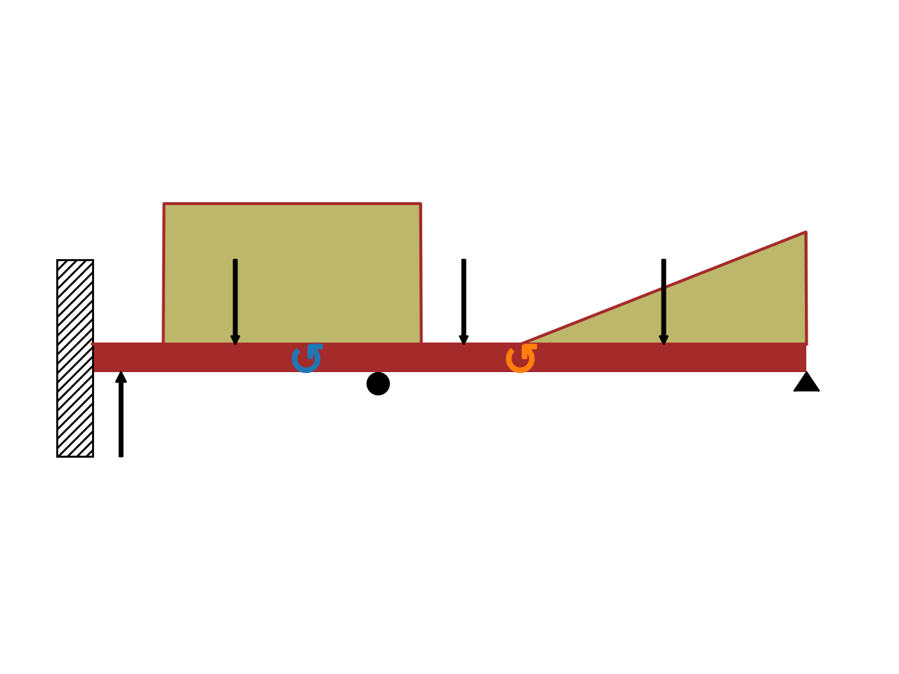
Returns a plot object representing the beam diagram of the beam. In particular, the diagram might include:
the beam.
vertical black arrows represent point loads and support reaction forces (the latter if they have been added with the
apply_loadmethod).circular arrows represent moments.
shaded areas represent distributed loads.
the support, if
apply_supporthas been executed.if a composite beam has been created with the
joinmethod and a hinge has been specified, it will be shown with a white disc.
The diagram shows positive loads on the upper side of the beam, and negative loads on the lower side. If two or more distributed loads acts along the same direction over the same region, the function will add them up together.
备注
The user must be careful while entering load values. The draw function assumes a sign convention which is used for plotting loads. Given a right handed coordinate system with XYZ coordinates, the beam's length is assumed to be along the positive X axis. The draw function recognizes positive loads(with n>-2) as loads acting along negative Y direction and positive moments acting along positive Z direction.
- 参数:
pictorial: Boolean (default=True)
Setting
pictorial=Truewould simply create a pictorial (scaled) view of the beam diagram. On the other hand,pictorial=Falsewould create a beam diagram with the exact dimensions on the plot.
实例
>>> from sympy.physics.continuum_mechanics.beam import Beam
>>> from sympy import symbols
>>> P1, P2, M = symbols('P1, P2, M')
>>> E, I = symbols('E, I')
>>> b = Beam(50, 20, 30)
>>> b.apply_load(-10, 2, -1)
>>> b.apply_load(15, 26, -1)
>>> b.apply_load(P1, 10, -1)
>>> b.apply_load(-P2, 40, -1)
>>> b.apply_load(90, 5, 0, 23)
>>> b.apply_load(10, 30, 1, 50)
>>> b.apply_load(M, 15, -2)
>>> b.apply_load(-M, 30, -2)
>>> b.apply_support(50, "pin")
>>> b.apply_support(0, "fixed")
>>> b.apply_support(20, "roller")
>>> p = b.draw()
>>> p
Plot object containing:
[0]: cartesian line: 25*SingularityFunction(x, 5, 0) - 25*SingularityFunction(x, 23, 0)
+ SingularityFunction(x, 30, 1) - 20*SingularityFunction(x, 50, 0)
- SingularityFunction(x, 50, 1) + 5 for x over (0.0, 50.0)
[1]: cartesian line: 5 for x over (0.0, 50.0)
...
>>> p.show()

- property elastic_modulus#
梁的杨氏模量。
- property ild_moment#
Returns the I.L.D. moment equation.
- property ild_reactions#
Returns the I.L.D. reaction forces in a dictionary.
- property ild_shear#
Returns the I.L.D. shear equation.
- join(beam, via='fixed')[源代码]#
这种方法将两个梁连接起来构成一个新的组合梁系统。传递的Beam类实例被附加到调用对象的右端。该方法可用于弹性模量或二阶矩不连续的梁。
- 参数:
beam :梁类对象
将连接到调用对象右侧的Beam对象。
via :字符串
说明两个光束对象的连接方式-对于轴向固定的梁,via=“fixed”-对于通过铰链连接的梁,via=“hinge”
实例
有一根4米长的悬臂梁。前2米的惯性矩为 \(1.5*I\) 和 \(I\) 另一方面。从其自由端的顶部施加4 N量级的点荷载。
>>> from sympy.physics.continuum_mechanics.beam import Beam
>>> from sympy import symbols
>>> E, I = symbols('E, I')
>>> R1, R2 = symbols('R1, R2')
>>> b1 = Beam(2, E, 1.5*I)
>>> b2 = Beam(2, E, I)
>>> b = b1.join(b2, "fixed")
>>> b.apply_load(20, 4, -1)
>>> b.apply_load(R1, 0, -1)
>>> b.apply_load(R2, 0, -2)
>>> b.bc_slope = [(0, 0)]
>>> b.bc_deflection = [(0, 0)]
>>> b.solve_for_reaction_loads(R1, R2)
>>> b.load
80*SingularityFunction(x, 0, -2) - 20*SingularityFunction(x, 0, -1) + 20*SingularityFunction(x, 4, -1)
>>> b.slope()
(-((-80*SingularityFunction(x, 0, 1) + 10*SingularityFunction(x, 0, 2) - 10*SingularityFunction(x, 4, 2))/I + 120/I)/E + 80.0/(E*I))*SingularityFunction(x, 2, 0)
- 0.666666666666667*(-80*SingularityFunction(x, 0, 1) + 10*SingularityFunction(x, 0, 2) - 10*SingularityFunction(x, 4, 2))*SingularityFunction(x, 0, 0)/(E*I)
+ 0.666666666666667*(-80*SingularityFunction(x, 0, 1) + 10*SingularityFunction(x, 0, 2) - 10*SingularityFunction(x, 4, 2))*SingularityFunction(x, 2, 0)/(E*I)
- property length#
梁的长度。
- property load#
返回表示梁对象的载荷分布曲线的奇异函数表达式。
实例
有一根4米长的横梁。在光束起始点处顺时针方向施加3 Nm的力矩。在距起点2米处从梁顶部施加4 N量级的点荷载,在距梁起点3米处的梁下方施加2 N/m的抛物线斜坡荷载。
>>> from sympy.physics.continuum_mechanics.beam import Beam
>>> from sympy import symbols
>>> E, I = symbols('E, I')
>>> b = Beam(4, E, I)
>>> b.apply_load(-3, 0, -2)
>>> b.apply_load(4, 2, -1)
>>> b.apply_load(-2, 3, 2)
>>> b.load
-3*SingularityFunction(x, 0, -2) + 4*SingularityFunction(x, 2, -1) - 2*SingularityFunction(x, 3, 2)
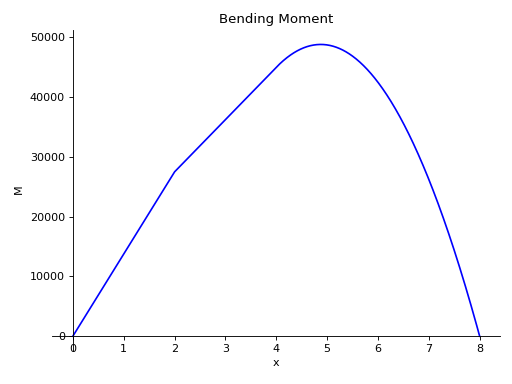
- plot_bending_moment(subs=None)[源代码]#
返回梁对象中存在的弯矩的绘图。
- 参数:
subs :字典
Python字典,包含作为键的符号及其相应的值。
实例
有一根8米长的横梁。从梁的一半到梁端施加10 KN/m的恒定分布荷载。在梁的下方有两个简支,一个在梁的起点,另一个在梁的终点。在距起点4米处,从梁顶部施加5 KN的点荷载。取E=200gpa,I=400 (10 -6) meter *4。
使用向下力为正的符号约定。
>>> from sympy.physics.continuum_mechanics.beam import Beam
>>> from sympy import symbols
>>> R1, R2 = symbols('R1, R2')
>>> b = Beam(8, 200*(10**9), 400*(10**-6))
>>> b.apply_load(5000, 2, -1)
>>> b.apply_load(R1, 0, -1)
>>> b.apply_load(R2, 8, -1)
>>> b.apply_load(10000, 4, 0, end=8)
>>> b.bc_deflection = [(0, 0), (8, 0)]
>>> b.solve_for_reaction_loads(R1, R2)
>>> b.plot_bending_moment()
Plot object containing:
[0]: cartesian line: 13750*SingularityFunction(x, 0, 1) - 5000*SingularityFunction(x, 2, 1)
- 5000*SingularityFunction(x, 4, 2) + 31250*SingularityFunction(x, 8, 1)
+ 5000*SingularityFunction(x, 8, 2) for x over (0.0, 8.0)

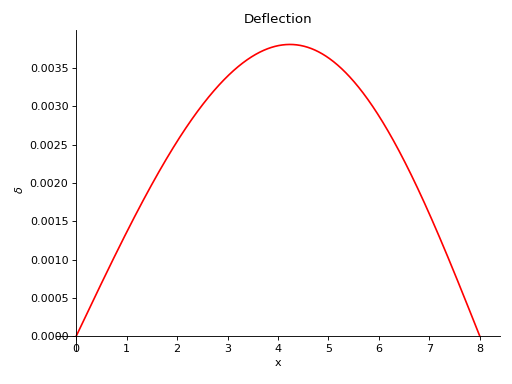
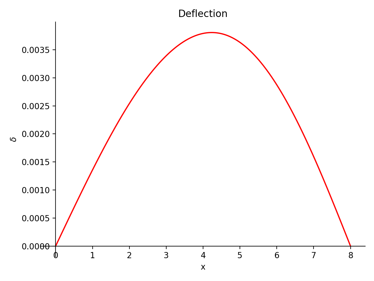
- plot_deflection(subs=None)[源代码]#
返回梁对象的挠度曲线图。
- 参数:
subs :字典
Python字典,包含作为键的符号及其相应的值。
实例
有一根8米长的横梁。从梁的一半到梁端施加10 KN/m的恒定分布荷载。在梁的下方有两个简支,一个在梁的起点,另一个在梁的终点。在距起点4米处,从梁顶部施加5 KN的点荷载。取E=200gpa,I=400 (10 -6) meter *4。
使用向下力为正的符号约定。
>>> from sympy.physics.continuum_mechanics.beam import Beam
>>> from sympy import symbols
>>> R1, R2 = symbols('R1, R2')
>>> b = Beam(8, 200*(10**9), 400*(10**-6))
>>> b.apply_load(5000, 2, -1)
>>> b.apply_load(R1, 0, -1)
>>> b.apply_load(R2, 8, -1)
>>> b.apply_load(10000, 4, 0, end=8)
>>> b.bc_deflection = [(0, 0), (8, 0)]
>>> b.solve_for_reaction_loads(R1, R2)
>>> b.plot_deflection()
Plot object containing:
[0]: cartesian line: 0.00138541666666667*x - 2.86458333333333e-5*SingularityFunction(x, 0, 3)
+ 1.04166666666667e-5*SingularityFunction(x, 2, 3) + 5.20833333333333e-6*SingularityFunction(x, 4, 4)
- 6.51041666666667e-5*SingularityFunction(x, 8, 3) - 5.20833333333333e-6*SingularityFunction(x, 8, 4)
for x over (0.0, 8.0)

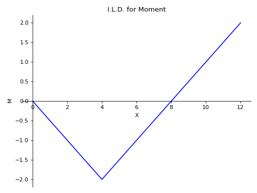
- plot_ild_moment(subs=None)[源代码]#
Plots the Influence Line Diagram for Moment under the effect of a moving load. This function should be called after calling solve_for_ild_moment().
- 参数:
subs :字典
Python字典,包含作为键的符号及其相应的值。
实例
There is a beam of length 12 meters. There are two simple supports below the beam, one at the starting point and another at a distance of 8 meters. Plot the I.L.D. for Moment at a distance of 4 meters under the effect of a moving load of magnitude 1kN.
使用向下力为正的符号约定。
>>> from sympy import symbols
>>> from sympy.physics.continuum_mechanics.beam import Beam
>>> E, I = symbols('E, I')
>>> R_0, R_8 = symbols('R_0, R_8')
>>> b = Beam(12, E, I)
>>> b.apply_support(0, 'roller')
>>> b.apply_support(8, 'roller')
>>> b.solve_for_ild_reactions(1, R_0, R_8)
>>> b.solve_for_ild_moment(4, 1, R_0, R_8)
>>> b.ild_moment
Piecewise((-x/2, x < 4), (x/2 - 4, x > 4))
>>> b.plot_ild_moment()
Plot object containing:
[0]: cartesian line: Piecewise((-x/2, x < 4), (x/2 - 4, x > 4)) for x over (0.0, 12.0)

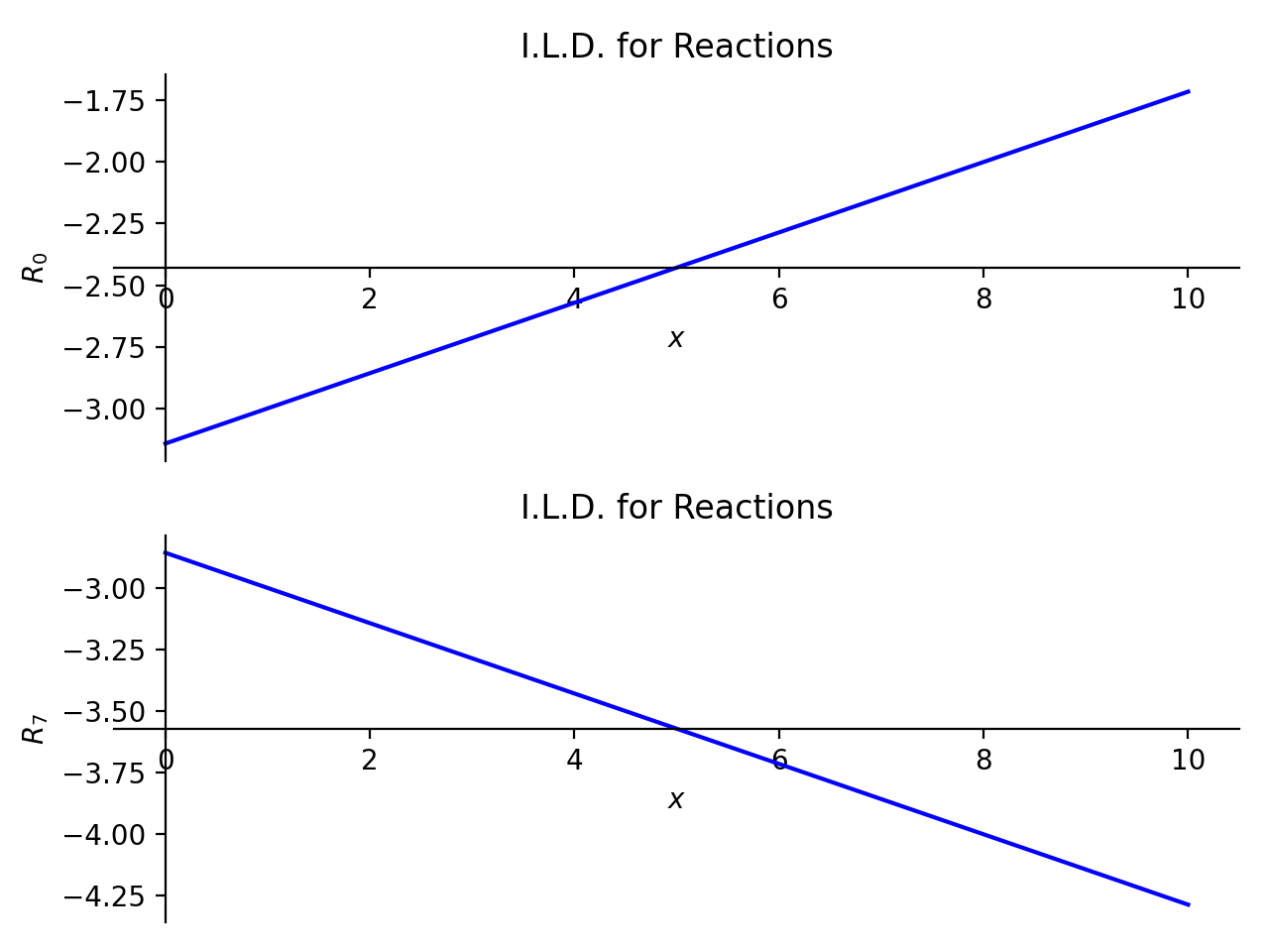
- plot_ild_reactions(subs=None)[源代码]#
Plots the Influence Line Diagram of Reaction Forces under the effect of a moving load. This function should be called after calling solve_for_ild_reactions().
- 参数:
subs :字典
Python字典,包含作为键的符号及其相应的值。
实例
There is a beam of length 10 meters. A point load of magnitude 5KN is also applied from top of the beam, at a distance of 4 meters from the starting point. There are two simple supports below the beam, located at the starting point and at a distance of 7 meters from the starting point. Plot the I.L.D. equations for reactions at both support points under the effect of a moving load of magnitude 1kN.
使用向下力为正的符号约定。
>>> from sympy import symbols
>>> from sympy.physics.continuum_mechanics.beam import Beam
>>> E, I = symbols('E, I')
>>> R_0, R_7 = symbols('R_0, R_7')
>>> b = Beam(10, E, I)
>>> b.apply_support(0, 'roller')
>>> b.apply_support(7, 'roller')
>>> b.apply_load(5,4,-1)
>>> b.solve_for_ild_reactions(1,R_0,R_7)
>>> b.ild_reactions
{R_0: x/7 - 22/7, R_7: -x/7 - 20/7}
>>> b.plot_ild_reactions()
PlotGrid object containing:
Plot[0]:Plot object containing:
[0]: cartesian line: x/7 - 22/7 for x over (0.0, 10.0)
Plot[1]:Plot object containing:
[0]: cartesian line: -x/7 - 20/7 for x over (0.0, 10.0)

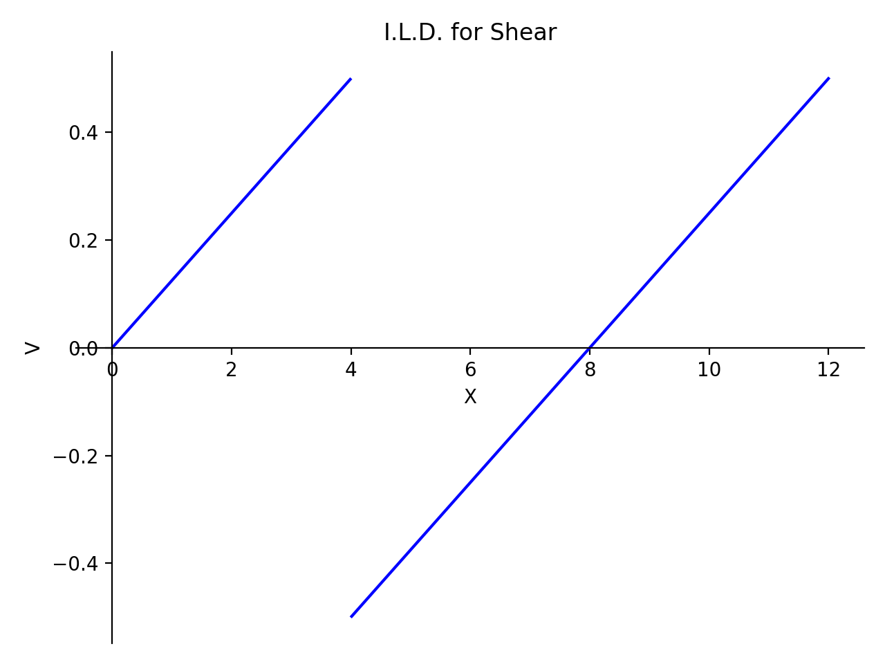
- plot_ild_shear(subs=None)[源代码]#
Plots the Influence Line Diagram for Shear under the effect of a moving load. This function should be called after calling solve_for_ild_shear().
- 参数:
subs :字典
Python字典,包含作为键的符号及其相应的值。
实例
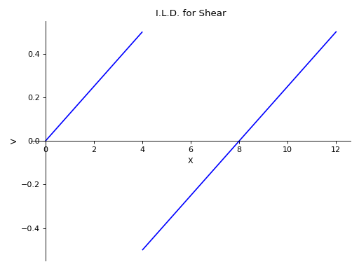
There is a beam of length 12 meters. There are two simple supports below the beam, one at the starting point and another at a distance of 8 meters. Plot the I.L.D. for Shear at a distance of 4 meters under the effect of a moving load of magnitude 1kN.
使用向下力为正的符号约定。
>>> from sympy import symbols
>>> from sympy.physics.continuum_mechanics.beam import Beam
>>> E, I = symbols('E, I')
>>> R_0, R_8 = symbols('R_0, R_8')
>>> b = Beam(12, E, I)
>>> b.apply_support(0, 'roller')
>>> b.apply_support(8, 'roller')
>>> b.solve_for_ild_reactions(1, R_0, R_8)
>>> b.solve_for_ild_shear(4, 1, R_0, R_8)
>>> b.ild_shear
Piecewise((x/8, x < 4), (x/8 - 1, x > 4))
>>> b.plot_ild_shear()
Plot object containing:
[0]: cartesian line: Piecewise((x/8, x < 4), (x/8 - 1, x > 4)) for x over (0.0, 12.0)
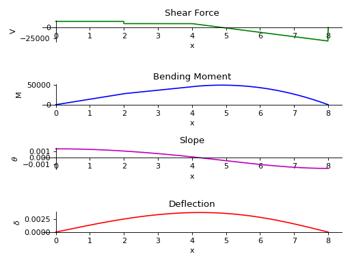
- plot_loading_results(subs=None)[源代码]#
返回梁对象的剪切力、弯矩、坡度和挠度的子批次。
- 参数:
subs :字典
Python字典,包含作为键的符号及其相应的值。
实例
有一根8米长的横梁。从梁的一半到梁端施加10 KN/m的恒定分布荷载。在梁的下方有两个简支,一个在梁的起点,另一个在梁的终点。在距起点4米处,从梁顶部施加5 KN的点荷载。取E=200gpa,I=400 (10 -6) meter *4。
使用向下力为正的符号约定。
>>> from sympy.physics.continuum_mechanics.beam import Beam
>>> from sympy import symbols
>>> R1, R2 = symbols('R1, R2')
>>> b = Beam(8, 200*(10**9), 400*(10**-6))
>>> b.apply_load(5000, 2, -1)
>>> b.apply_load(R1, 0, -1)
>>> b.apply_load(R2, 8, -1)
>>> b.apply_load(10000, 4, 0, end=8)
>>> b.bc_deflection = [(0, 0), (8, 0)]
>>> b.solve_for_reaction_loads(R1, R2)
>>> axes = b.plot_loading_results()

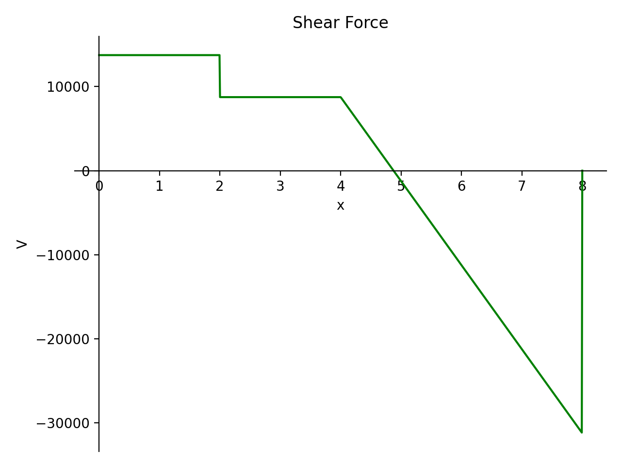
- plot_shear_force(subs=None)[源代码]#
返回梁对象中存在的剪切力的绘图。
- 参数:
subs :字典
Python字典,包含作为键的符号及其相应的值。
实例
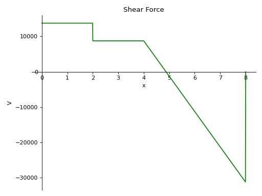
有一根8米长的横梁。从梁的一半到梁端施加10 KN/m的恒定分布荷载。在梁的下方有两个简支,一个在梁的起点,另一个在梁的终点。在距起点4米处,从梁顶部施加5 KN的点荷载。取E=200gpa,I=400 (10 -6) meter *4。
使用向下力为正的符号约定。
>>> from sympy.physics.continuum_mechanics.beam import Beam
>>> from sympy import symbols
>>> R1, R2 = symbols('R1, R2')
>>> b = Beam(8, 200*(10**9), 400*(10**-6))
>>> b.apply_load(5000, 2, -1)
>>> b.apply_load(R1, 0, -1)
>>> b.apply_load(R2, 8, -1)
>>> b.apply_load(10000, 4, 0, end=8)
>>> b.bc_deflection = [(0, 0), (8, 0)]
>>> b.solve_for_reaction_loads(R1, R2)
>>> b.plot_shear_force()
Plot object containing:
[0]: cartesian line: 13750*SingularityFunction(x, 0, 0) - 5000*SingularityFunction(x, 2, 0)
- 10000*SingularityFunction(x, 4, 1) + 31250*SingularityFunction(x, 8, 0)
+ 10000*SingularityFunction(x, 8, 1) for x over (0.0, 8.0)
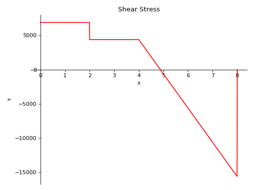
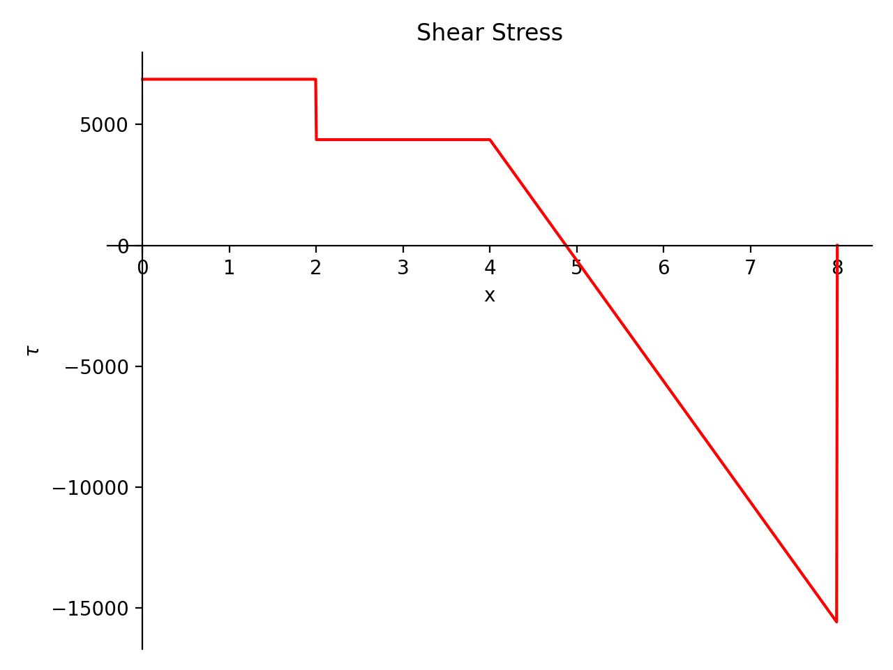
- plot_shear_stress(subs=None)[源代码]#
Returns a plot of shear stress present in the beam object.
- 参数:
subs :字典
Python字典,包含作为键的符号及其相应的值。
实例
There is a beam of length 8 meters and area of cross section 2 square meters. A constant distributed load of 10 KN/m is applied from half of the beam till the end. There are two simple supports below the beam, one at the starting point and another at the ending point of the beam. A pointload of magnitude 5 KN is also applied from top of the beam, at a distance of 4 meters from the starting point. Take E = 200 GPa and I = 400*(10**-6) meter**4.
使用向下力为正的符号约定。
>>> from sympy.physics.continuum_mechanics.beam import Beam
>>> from sympy import symbols
>>> R1, R2 = symbols('R1, R2')
>>> b = Beam(8, 200*(10**9), 400*(10**-6), 2)
>>> b.apply_load(5000, 2, -1)
>>> b.apply_load(R1, 0, -1)
>>> b.apply_load(R2, 8, -1)
>>> b.apply_load(10000, 4, 0, end=8)
>>> b.bc_deflection = [(0, 0), (8, 0)]
>>> b.solve_for_reaction_loads(R1, R2)
>>> b.plot_shear_stress()
Plot object containing:
[0]: cartesian line: 6875*SingularityFunction(x, 0, 0) - 2500*SingularityFunction(x, 2, 0)
- 5000*SingularityFunction(x, 4, 1) + 15625*SingularityFunction(x, 8, 0)
+ 5000*SingularityFunction(x, 8, 1) for x over (0.0, 8.0)

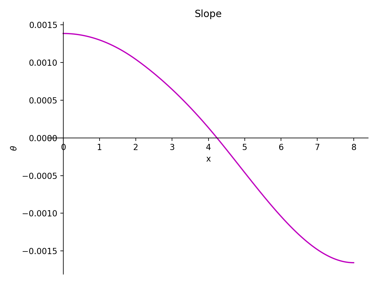
- plot_slope(subs=None)[源代码]#
返回梁对象的偏转曲线斜率的绘图。
- 参数:
subs :字典
Python字典,包含作为键的符号及其相应的值。
实例
有一根8米长的横梁。从梁的一半到梁端施加10 KN/m的恒定分布荷载。在梁的下方有两个简支,一个在梁的起点,另一个在梁的终点。在距起点4米处,从梁顶部施加5 KN的点荷载。取E=200gpa,I=400 (10 -6) meter *4。
使用向下力为正的符号约定。
>>> from sympy.physics.continuum_mechanics.beam import Beam
>>> from sympy import symbols
>>> R1, R2 = symbols('R1, R2')
>>> b = Beam(8, 200*(10**9), 400*(10**-6))
>>> b.apply_load(5000, 2, -1)
>>> b.apply_load(R1, 0, -1)
>>> b.apply_load(R2, 8, -1)
>>> b.apply_load(10000, 4, 0, end=8)
>>> b.bc_deflection = [(0, 0), (8, 0)]
>>> b.solve_for_reaction_loads(R1, R2)
>>> b.plot_slope()
Plot object containing:
[0]: cartesian line: -8.59375e-5*SingularityFunction(x, 0, 2) + 3.125e-5*SingularityFunction(x, 2, 2)
+ 2.08333333333333e-5*SingularityFunction(x, 4, 3) - 0.0001953125*SingularityFunction(x, 8, 2)
- 2.08333333333333e-5*SingularityFunction(x, 8, 3) + 0.00138541666666667 for x over (0.0, 8.0)

- point_cflexure()[源代码]#
返回一组弯矩为零的点,其中梁对象的弯矩曲线的符号从负变为正,反之亦然。
实例
有10米长的悬挑梁。横梁下面有两个简单的支架。一个在起点,另一个在距起点6米的地方。分别在距起点2米和4米处施加10KN和20KN的点荷载。在距起点6米处至终点的顶部施加3KN/m量级的均匀分布荷载。使用向上力和顺时针力矩为正的符号惯例。
>>> from sympy.physics.continuum_mechanics.beam import Beam
>>> from sympy import symbols
>>> E, I = symbols('E, I')
>>> b = Beam(10, E, I)
>>> b.apply_load(-4, 0, -1)
>>> b.apply_load(-46, 6, -1)
>>> b.apply_load(10, 2, -1)
>>> b.apply_load(20, 4, -1)
>>> b.apply_load(3, 6, 0)
>>> b.point_cflexure()
[10/3]
- property reaction_loads#
返回字典中的反作用力。
- remove_load(value, start, order, end=None)[源代码]#
此方法将删除梁对象上存在的特定载荷。如果梁上不存在作为参数传递的载荷,则返回ValueError。
- 参数:
价值 :可解释
施加荷载的大小。
开始 :可解释
施加荷载的起点。对于点力矩和点力,这是应用的位置。
秩序 :整数
施加荷载的顺序。-对于力矩,顺序=-2-对于点荷载,顺序=-1-对于恒定分布荷载,顺序=0-对于斜坡荷载,顺序=1-对于抛物线斜坡荷载,顺序=2-。。。等等。
end :可解释,可选
如果荷载的终点在梁的长度内,则可以使用此可选参数。
实例
有一根4米长的横梁。在光束起始点处顺时针方向施加3 Nm的力矩。在距起点2米处从梁顶部施加4 N量级的点荷载,在距梁起点2米至3米处的梁下方施加2 N/m量级的抛物线斜坡荷载。
>>> from sympy.physics.continuum_mechanics.beam import Beam
>>> from sympy import symbols
>>> E, I = symbols('E, I')
>>> b = Beam(4, E, I)
>>> b.apply_load(-3, 0, -2)
>>> b.apply_load(4, 2, -1)
>>> b.apply_load(-2, 2, 2, end=3)
>>> b.load
-3*SingularityFunction(x, 0, -2) + 4*SingularityFunction(x, 2, -1) - 2*SingularityFunction(x, 2, 2) + 2*SingularityFunction(x, 3, 0) + 4*SingularityFunction(x, 3, 1) + 2*SingularityFunction(x, 3, 2)
>>> b.remove_load(-2, 2, 2, end = 3)
>>> b.load
-3*SingularityFunction(x, 0, -2) + 4*SingularityFunction(x, 2, -1)
- property second_moment#
梁面积的二阶矩。
- shear_force()[源代码]#
返回表示梁对象剪切力曲线的奇异函数表达式。
实例
有一根30米长的横梁。在光束末端顺时针方向施加120牛米的力矩。在起点处从梁顶部施加8 N的点荷载。横梁下面有两个简单的支架。一个在终点,另一个在距起点10米的地方。挠度在两个支座处都受到限制。
使用向上力和顺时针力矩为正的符号惯例。
>>> from sympy.physics.continuum_mechanics.beam import Beam
>>> from sympy import symbols
>>> E, I = symbols('E, I')
>>> R1, R2 = symbols('R1, R2')
>>> b = Beam(30, E, I)
>>> b.apply_load(-8, 0, -1)
>>> b.apply_load(R1, 10, -1)
>>> b.apply_load(R2, 30, -1)
>>> b.apply_load(120, 30, -2)
>>> b.bc_deflection = [(10, 0), (30, 0)]
>>> b.solve_for_reaction_loads(R1, R2)
>>> b.shear_force()
8*SingularityFunction(x, 0, 0) - 6*SingularityFunction(x, 10, 0) - 120*SingularityFunction(x, 30, -1) - 2*SingularityFunction(x, 30, 0)
- slope()[源代码]#
返回一个奇点函数表达式,该表达式表示梁对象的弹性曲线的斜率。
实例
有一根30米长的横梁。在光束末端顺时针方向施加120牛米的力矩。在起点处从梁顶部施加8 N的点荷载。横梁下面有两个简单的支架。一个在终点,另一个在距起点10米的地方。挠度在两个支座处都受到限制。
使用向上力和顺时针力矩为正的符号惯例。
>>> from sympy.physics.continuum_mechanics.beam import Beam
>>> from sympy import symbols
>>> E, I = symbols('E, I')
>>> R1, R2 = symbols('R1, R2')
>>> b = Beam(30, E, I)
>>> b.apply_load(-8, 0, -1)
>>> b.apply_load(R1, 10, -1)
>>> b.apply_load(R2, 30, -1)
>>> b.apply_load(120, 30, -2)
>>> b.bc_deflection = [(10, 0), (30, 0)]
>>> b.solve_for_reaction_loads(R1, R2)
>>> b.slope()
(-4*SingularityFunction(x, 0, 2) + 3*SingularityFunction(x, 10, 2)
    + 120*SingularityFunction(x, 30, 1) + SingularityFunction(x, 30, 2) + 4000/3)/(E*I)
- solve_for_ild_moment(distance, value, *reactions)[源代码]#
Determines the Influence Line Diagram equations for moment at a specified point under the effect of a moving load.
- 参数:
distance : Integer
Distance of the point from the start of the beam for which equations are to be determined
value : Integer
Magnitude of moving load
reactions :
The reaction forces applied on the beam.
实例
There is a beam of length 12 meters. There are two simple supports below the beam, one at the starting point and another at a distance of 8 meters. Calculate the I.L.D. equations for Moment at a distance of 4 meters under the effect of a moving load of magnitude 1kN.
使用向下力为正的符号约定。
>>> from sympy import symbols
>>> from sympy.physics.continuum_mechanics.beam import Beam
>>> E, I = symbols('E, I')
>>> R_0, R_8 = symbols('R_0, R_8')
>>> b = Beam(12, E, I)
>>> b.apply_support(0, 'roller')
>>> b.apply_support(8, 'roller')
>>> b.solve_for_ild_reactions(1, R_0, R_8)
>>> b.solve_for_ild_moment(4, 1, R_0, R_8)
>>> b.ild_moment
Piecewise((-x/2, x < 4), (x/2 - 4, x > 4))
- solve_for_ild_reactions(value, *reactions)[源代码]#
Determines the Influence Line Diagram equations for reaction forces under the effect of a moving load.
- 参数:
value : Integer
Magnitude of moving load
reactions :
The reaction forces applied on the beam.
实例
There is a beam of length 10 meters. There are two simple supports below the beam, one at the starting point and another at the ending point of the beam. Calculate the I.L.D. equations for reaction forces under the effect of a moving load of magnitude 1kN.
使用向下力为正的符号约定。
>>> from sympy import symbols
>>> from sympy.physics.continuum_mechanics.beam import Beam
>>> E, I = symbols('E, I')
>>> R_0, R_10 = symbols('R_0, R_10')
>>> b = Beam(10, E, I)
>>> b.apply_support(0, 'roller')
>>> b.apply_support(10, 'roller')
>>> b.solve_for_ild_reactions(1,R_0,R_10)
>>> b.ild_reactions
{R_0: x/10 - 1, R_10: -x/10}
- solve_for_ild_shear(distance, value, *reactions)[源代码]#
Determines the Influence Line Diagram equations for shear at a specified point under the effect of a moving load.
- 参数:
distance : Integer
Distance of the point from the start of the beam for which equations are to be determined
value : Integer
Magnitude of moving load
reactions :
The reaction forces applied on the beam.
实例
There is a beam of length 12 meters. There are two simple supports below the beam, one at the starting point and another at a distance of 8 meters. Calculate the I.L.D. equations for Shear at a distance of 4 meters under the effect of a moving load of magnitude 1kN.
使用向下力为正的符号约定。
>>> from sympy import symbols
>>> from sympy.physics.continuum_mechanics.beam import Beam
>>> E, I = symbols('E, I')
>>> R_0, R_8 = symbols('R_0, R_8')
>>> b = Beam(12, E, I)
>>> b.apply_support(0, 'roller')
>>> b.apply_support(8, 'roller')
>>> b.solve_for_ild_reactions(1, R_0, R_8)
>>> b.solve_for_ild_shear(4, 1, R_0, R_8)
>>> b.ild_shear
Piecewise((x/8, x < 4), (x/8 - 1, x > 4))
- solve_for_reaction_loads(*reactions)[源代码]#
求解反作用力。
实例
有一根30米长的横梁。在光束末端顺时针方向施加120牛米的力矩。在起点处从梁顶部施加8 N的点荷载。横梁下面有两个简单的支架。一个在终点,另一个在距起点10米的地方。挠度在两个支座处都受到限制。
使用向上力和顺时针力矩为正的符号惯例。
>>> from sympy.physics.continuum_mechanics.beam import Beam
>>> from sympy import symbols
>>> E, I = symbols('E, I')
>>> R1, R2 = symbols('R1, R2')
>>> b = Beam(30, E, I)
>>> b.apply_load(-8, 0, -1)
>>> b.apply_load(R1, 10, -1)  # Reaction force at x = 10
>>> b.apply_load(R2, 30, -1)  # Reaction force at x = 30
>>> b.apply_load(120, 30, -2)
>>> b.bc_deflection = [(10, 0), (30, 0)]
>>> b.load
R1*SingularityFunction(x, 10, -1) + R2*SingularityFunction(x, 30, -1)
    - 8*SingularityFunction(x, 0, -1) + 120*SingularityFunction(x, 30, -2)
>>> b.solve_for_reaction_loads(R1, R2)
>>> b.reaction_loads
{R1: 6, R2: 2}
>>> b.load
-8*SingularityFunction(x, 0, -1) + 6*SingularityFunction(x, 10, -1)
    + 120*SingularityFunction(x, 30, -2) + 2*SingularityFunction(x, 30, -1)
- property variable#
在表示荷载分布、剪力曲线、弯矩、坡度曲线和挠度曲线时,可作为梁长度的变量使用的符号。默认设置为
Symbol('x'),但此属性是可变的。实例
>>> from sympy.physics.continuum_mechanics.beam import Beam
>>> from sympy import symbols
>>> E, I, A = symbols('E, I, A')
>>> x, y, z = symbols('x, y, z')
>>> b = Beam(4, E, I)
>>> b.variable
x
>>> b.variable = y
>>> b.variable
y
>>> b = Beam(4, E, I, A, z)
>>> b.variable
z
- class sympy.physics.continuum_mechanics.beam.Beam3D(length, elastic_modulus, shear_modulus, second_moment, area, variable=x)[源代码]#
此类处理应用于三维空间任何方向的载荷,以及沿不同轴的第二力矩不相等的值。
备注
A consistent sign convention must be used while solving a beam bending problem; the results will automatically follow the chosen sign convention. This class assumes that any kind of distributed load/moment is applied through out the span of a beam.
实例
有一根1米长的横梁。从梁开始到梁端,沿y轴施加一个q量级的恒定分布荷载。从梁开始到梁端,沿z轴施加一个m量级的恒定分布力矩。横梁两端固定。因此,两端梁的挠度受到限制。
>>> from sympy.physics.continuum_mechanics.beam import Beam3D
>>> from sympy import symbols, simplify, collect, factor
>>> l, E, G, I, A = symbols('l, E, G, I, A')
>>> b = Beam3D(l, E, G, I, A)
>>> x, q, m = symbols('x, q, m')
>>> b.apply_load(q, 0, 0, dir="y")
>>> b.apply_moment_load(m, 0, -1, dir="z")
>>> b.shear_force()
[0, -q*x, 0]
>>> b.bending_moment()
[0, 0, -m*x + q*x**2/2]
>>> b.bc_slope = [(0, [0, 0, 0]), (l, [0, 0, 0])]
>>> b.bc_deflection = [(0, [0, 0, 0]), (l, [0, 0, 0])]
>>> b.solve_slope_deflection()
>>> factor(b.slope())
[0, 0, x*(-l + x)*(-A*G*l**3*q + 2*A*G*l**2*q*x - 12*E*I*l*q
    - 72*E*I*m + 24*E*I*q*x)/(12*E*I*(A*G*l**2 + 12*E*I))]
>>> dx, dy, dz = b.deflection()
>>> dy = collect(simplify(dy), x)
>>> dx == dz == 0
True
>>> dy == (x*(12*E*I*l*(A*G*l**2*q - 2*A*G*l*m + 12*E*I*q)
... + x*(A*G*l*(3*l*(A*G*l**2*q - 2*A*G*l*m + 12*E*I*q) + x*(-2*A*G*l**2*q + 4*A*G*l*m - 24*E*I*q))
... + A*G*(A*G*l**2 + 12*E*I)*(-2*l**2*q + 6*l*m - 4*m*x + q*x**2)
... - 12*E*I*q*(A*G*l**2 + 12*E*I)))/(24*A*E*G*I*(A*G*l**2 + 12*E*I)))
True
工具书类
- angular_deflection()[源代码]#
Returns a function in x depicting how the angular deflection, due to moments in the x-axis on the beam, varies with x.
- apply_load(value, start, order, dir='y')[源代码]#
此方法将力载荷加到特定的梁对象上。
- 参数:
价值 :可解释
施加荷载的大小。
dir :字符串
施加荷载的轴。
秩序 :整数
施加荷载的顺序。-对于点荷载,顺序=-1-对于恒定分布荷载,顺序=0-对于斜坡荷载,顺序=1-对于抛物线斜坡荷载,顺序=2-。。。等等。
- apply_moment_load(value, start, order, dir='y')[源代码]#
此方法将力矩载荷相加到特定梁对象。
- 参数:
价值 :可解释
施加力矩的大小。
dir :字符串
施加力矩的轴。
秩序 :整数
施加荷载的顺序。-对于点力矩,顺序=-2-对于恒定分布力矩,顺序=-1-对于斜坡力矩,顺序=0-对于抛物线斜坡力矩,顺序=1-。。。等等。
- property area#
梁的横截面积。
- property boundary_conditions#
返回应用于梁的边界条件字典。这本词典有两个关键字,即斜率和挠度。每个关键字的值是一个元组列表,其中每个元组包含格式为(location,value)的边界条件的位置和值。此外,每个值是对应于该位置三个轴上的坡度或挠度值的列表。
实例
有一根4米长的横梁。0处的坡度沿x轴应为4,沿其他轴应为0。在梁的另一端,沿三个轴的挠度应为零。
>>> from sympy.physics.continuum_mechanics.beam import Beam3D
>>> from sympy import symbols
>>> l, E, G, I, A, x = symbols('l, E, G, I, A, x')
>>> b = Beam3D(30, E, G, I, A, x)
>>> b.bc_slope = [(0, (4, 0, 0))]
>>> b.bc_deflection = [(4, [0, 0, 0])]
>>> b.boundary_conditions
{'deflection': [(4, [0, 0, 0])], 'slope': [(0, (4, 0, 0))]}
这里梁的挠度应该是
0沿着三条轴线4. 同样,梁的坡度应为4沿x轴和0沿y轴和z轴0.
- property load_vector#
返回表示加载向量的三元素列表。
- max_bending_moment()[源代码]#
Returns point of max bending moment and its corresponding bending moment value along all directions in a Beam object as a list. solve_for_reaction_loads() must be called before using this function.
实例
There is a beam of length 20 meters. It is supported by rollers at both of its ends. A linear load having slope equal to 12 is applied along y-axis. A constant distributed load of magnitude 15 N is applied from start till its end along z-axis.
>>> from sympy.physics.continuum_mechanics.beam import Beam3D
>>> from sympy import symbols
>>> l, E, G, I, A, x = symbols('l, E, G, I, A, x')
>>> b = Beam3D(20, 40, 21, 100, 25, x)
>>> b.apply_load(15, start=0, order=0, dir="z")
>>> b.apply_load(12*x, start=0, order=0, dir="y")
>>> b.bc_deflection = [(0, [0, 0, 0]), (20, [0, 0, 0])]
>>> R1, R2, R3, R4 = symbols('R1, R2, R3, R4')
>>> b.apply_load(R1, start=0, order=-1, dir="z")
>>> b.apply_load(R2, start=20, order=-1, dir="z")
>>> b.apply_load(R3, start=0, order=-1, dir="y")
>>> b.apply_load(R4, start=20, order=-1, dir="y")
>>> b.solve_for_reaction_loads(R1, R2, R3, R4)
>>> b.max_bending_moment()
[(0, 0), (20, 3000), (20, 16000)]
- max_bmoment()[源代码]#
Returns point of max bending moment and its corresponding bending moment value along all directions in a Beam object as a list. solve_for_reaction_loads() must be called before using this function.
实例
There is a beam of length 20 meters. It is supported by rollers at both of its ends. A linear load having slope equal to 12 is applied along y-axis. A constant distributed load of magnitude 15 N is applied from start till its end along z-axis.
>>> from sympy.physics.continuum_mechanics.beam import Beam3D
>>> from sympy import symbols
>>> l, E, G, I, A, x = symbols('l, E, G, I, A, x')
>>> b = Beam3D(20, 40, 21, 100, 25, x)
>>> b.apply_load(15, start=0, order=0, dir="z")
>>> b.apply_load(12*x, start=0, order=0, dir="y")
>>> b.bc_deflection = [(0, [0, 0, 0]), (20, [0, 0, 0])]
>>> R1, R2, R3, R4 = symbols('R1, R2, R3, R4')
>>> b.apply_load(R1, start=0, order=-1, dir="z")
>>> b.apply_load(R2, start=20, order=-1, dir="z")
>>> b.apply_load(R3, start=0, order=-1, dir="y")
>>> b.apply_load(R4, start=20, order=-1, dir="y")
>>> b.solve_for_reaction_loads(R1, R2, R3, R4)
>>> b.max_bending_moment()
[(0, 0), (20, 3000), (20, 16000)]
- max_deflection()[源代码]#
Returns point of max deflection and its corresponding deflection value along all directions in a Beam object as a list. solve_for_reaction_loads() and solve_slope_deflection() must be called before using this function.
实例
There is a beam of length 20 meters. It is supported by rollers at both of its ends. A linear load having slope equal to 12 is applied along y-axis. A constant distributed load of magnitude 15 N is applied from start till its end along z-axis.
>>> from sympy.physics.continuum_mechanics.beam import Beam3D
>>> from sympy import symbols
>>> l, E, G, I, A, x = symbols('l, E, G, I, A, x')
>>> b = Beam3D(20, 40, 21, 100, 25, x)
>>> b.apply_load(15, start=0, order=0, dir="z")
>>> b.apply_load(12*x, start=0, order=0, dir="y")
>>> b.bc_deflection = [(0, [0, 0, 0]), (20, [0, 0, 0])]
>>> R1, R2, R3, R4 = symbols('R1, R2, R3, R4')
>>> b.apply_load(R1, start=0, order=-1, dir="z")
>>> b.apply_load(R2, start=20, order=-1, dir="z")
>>> b.apply_load(R3, start=0, order=-1, dir="y")
>>> b.apply_load(R4, start=20, order=-1, dir="y")
>>> b.solve_for_reaction_loads(R1, R2, R3, R4)
>>> b.solve_slope_deflection()
>>> b.max_deflection()
[(0, 0), (10, 495/14), (-10 + 10*sqrt(10793)/43, (10 - 10*sqrt(10793)/43)**3/160 - 20/7 + (10 - 10*sqrt(10793)/43)**4/6400 + 20*sqrt(10793)/301 + 27*(10 - 10*sqrt(10793)/43)**2/560)]
- max_shear_force()[源代码]#
Returns point of max shear force and its corresponding shear value along all directions in a Beam object as a list. solve_for_reaction_loads() must be called before using this function.
实例
There is a beam of length 20 meters. It is supported by rollers at both of its ends. A linear load having slope equal to 12 is applied along y-axis. A constant distributed load of magnitude 15 N is applied from start till its end along z-axis.
>>> from sympy.physics.continuum_mechanics.beam import Beam3D
>>> from sympy import symbols
>>> l, E, G, I, A, x = symbols('l, E, G, I, A, x')
>>> b = Beam3D(20, 40, 21, 100, 25, x)
>>> b.apply_load(15, start=0, order=0, dir="z")
>>> b.apply_load(12*x, start=0, order=0, dir="y")
>>> b.bc_deflection = [(0, [0, 0, 0]), (20, [0, 0, 0])]
>>> R1, R2, R3, R4 = symbols('R1, R2, R3, R4')
>>> b.apply_load(R1, start=0, order=-1, dir="z")
>>> b.apply_load(R2, start=20, order=-1, dir="z")
>>> b.apply_load(R3, start=0, order=-1, dir="y")
>>> b.apply_load(R4, start=20, order=-1, dir="y")
>>> b.solve_for_reaction_loads(R1, R2, R3, R4)
>>> b.max_shear_force()
[(0, 0), (20, 2400), (20, 300)]
- property moment_load_vector#
返回表示梁上的力矩载荷的三元素列表。
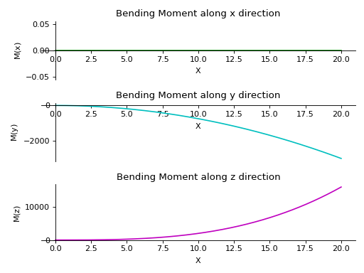
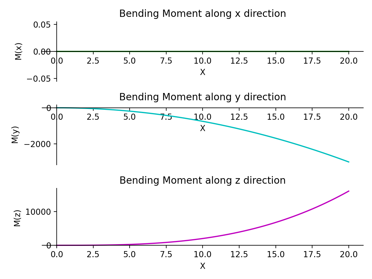
- plot_bending_moment(dir='all', subs=None)[源代码]#
Returns a plot for bending moment along all three directions present in the Beam object.
- 参数:
dir : string (default
Direction along which bending moment plot is required. If no direction is specified, all plots are displayed.
subs :字典
Python字典,包含作为键的符号及其相应的值。
实例
There is a beam of length 20 meters. It is supported by rollers at both of its ends. A linear load having slope equal to 12 is applied along y-axis. A constant distributed load of magnitude 15 N is applied from start till its end along z-axis.
>>> from sympy.physics.continuum_mechanics.beam import Beam3D
>>> from sympy import symbols
>>> l, E, G, I, A, x = symbols('l, E, G, I, A, x')
>>> b = Beam3D(20, E, G, I, A, x)
>>> b.apply_load(15, start=0, order=0, dir="z")
>>> b.apply_load(12*x, start=0, order=0, dir="y")
>>> b.bc_deflection = [(0, [0, 0, 0]), (20, [0, 0, 0])]
>>> R1, R2, R3, R4 = symbols('R1, R2, R3, R4')
>>> b.apply_load(R1, start=0, order=-1, dir="z")
>>> b.apply_load(R2, start=20, order=-1, dir="z")
>>> b.apply_load(R3, start=0, order=-1, dir="y")
>>> b.apply_load(R4, start=20, order=-1, dir="y")
>>> b.solve_for_reaction_loads(R1, R2, R3, R4)
>>> b.plot_bending_moment()
PlotGrid object containing:
Plot[0]:Plot object containing:
[0]: cartesian line: 0 for x over (0.0, 20.0)
Plot[1]:Plot object containing:
[0]: cartesian line: -15*x**2/2 for x over (0.0, 20.0)
Plot[2]:Plot object containing:
[0]: cartesian line: 2*x**3 for x over (0.0, 20.0)

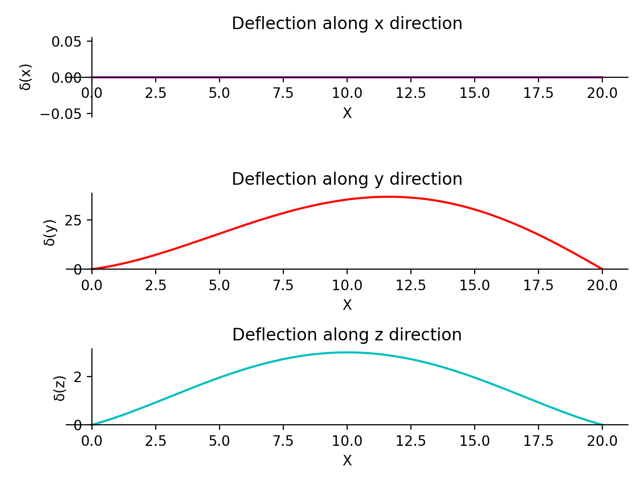
- plot_deflection(dir='all', subs=None)[源代码]#
Returns a plot for Deflection along all three directions present in the Beam object.
- 参数:
dir : string (default
Direction along which deflection plot is required. If no direction is specified, all plots are displayed.
subs :字典
Python dictionary containing Symbols as keys and their corresponding values.
实例
There is a beam of length 20 meters. It is supported by rollers at both of its ends. A linear load having slope equal to 12 is applied along y-axis. A constant distributed load of magnitude 15 N is applied from start till its end along z-axis.
>>> from sympy.physics.continuum_mechanics.beam import Beam3D
>>> from sympy import symbols
>>> l, E, G, I, A, x = symbols('l, E, G, I, A, x')
>>> b = Beam3D(20, 40, 21, 100, 25, x)
>>> b.apply_load(15, start=0, order=0, dir="z")
>>> b.apply_load(12*x, start=0, order=0, dir="y")
>>> b.bc_deflection = [(0, [0, 0, 0]), (20, [0, 0, 0])]
>>> R1, R2, R3, R4 = symbols('R1, R2, R3, R4')
>>> b.apply_load(R1, start=0, order=-1, dir="z")
>>> b.apply_load(R2, start=20, order=-1, dir="z")
>>> b.apply_load(R3, start=0, order=-1, dir="y")
>>> b.apply_load(R4, start=20, order=-1, dir="y")
>>> b.solve_for_reaction_loads(R1, R2, R3, R4)
>>> b.solve_slope_deflection()
>>> b.plot_deflection()
PlotGrid object containing:
Plot[0]:Plot object containing:
[0]: cartesian line: 0 for x over (0.0, 20.0)
Plot[1]:Plot object containing:
[0]: cartesian line: x**5/40000 - 4013*x**3/90300 + 26*x**2/43 + 1520*x/903 for x over (0.0, 20.0)
Plot[2]:Plot object containing:
[0]: cartesian line: x**4/6400 - x**3/160 + 27*x**2/560 + 2*x/7 for x over (0.0, 20.0)

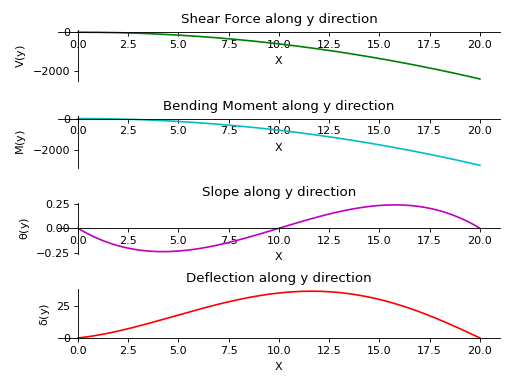
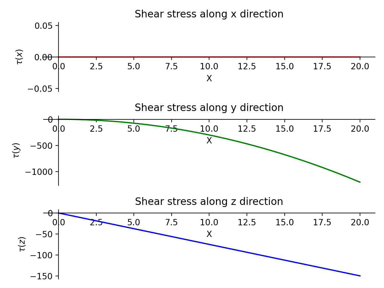
- plot_loading_results(dir='x', subs=None)[源代码]#
Returns a subplot of Shear Force, Bending Moment, Slope and Deflection of the Beam object along the direction specified.
- 参数:
dir : string (default
Direction along which plots are required. If no direction is specified, plots along x-axis are displayed.
subs :字典
Python字典,包含作为键的符号及其相应的值。
实例
There is a beam of length 20 meters. It is supported by rollers at both of its ends. A linear load having slope equal to 12 is applied along y-axis. A constant distributed load of magnitude 15 N is applied from start till its end along z-axis.
>>> from sympy.physics.continuum_mechanics.beam import Beam3D
>>> from sympy import symbols
>>> l, E, G, I, A, x = symbols('l, E, G, I, A, x')
>>> b = Beam3D(20, E, G, I, A, x)
>>> subs = {E:40, G:21, I:100, A:25}
>>> b.apply_load(15, start=0, order=0, dir="z")
>>> b.apply_load(12*x, start=0, order=0, dir="y")
>>> b.bc_deflection = [(0, [0, 0, 0]), (20, [0, 0, 0])]
>>> R1, R2, R3, R4 = symbols('R1, R2, R3, R4')
>>> b.apply_load(R1, start=0, order=-1, dir="z")
>>> b.apply_load(R2, start=20, order=-1, dir="z")
>>> b.apply_load(R3, start=0, order=-1, dir="y")
>>> b.apply_load(R4, start=20, order=-1, dir="y")
>>> b.solve_for_reaction_loads(R1, R2, R3, R4)
>>> b.solve_slope_deflection()
>>> b.plot_loading_results('y',subs)
PlotGrid object containing:
Plot[0]:Plot object containing:
[0]: cartesian line: -6*x**2 for x over (0.0, 20.0)
Plot[1]:Plot object containing:
[0]: cartesian line: -15*x**2/2 for x over (0.0, 20.0)
Plot[2]:Plot object containing:
[0]: cartesian line: -x**3/1600 + 3*x**2/160 - x/8 for x over (0.0, 20.0)
Plot[3]:Plot object containing:
[0]: cartesian line: x**5/40000 - 4013*x**3/90300 + 26*x**2/43 + 1520*x/903 for x over (0.0, 20.0)

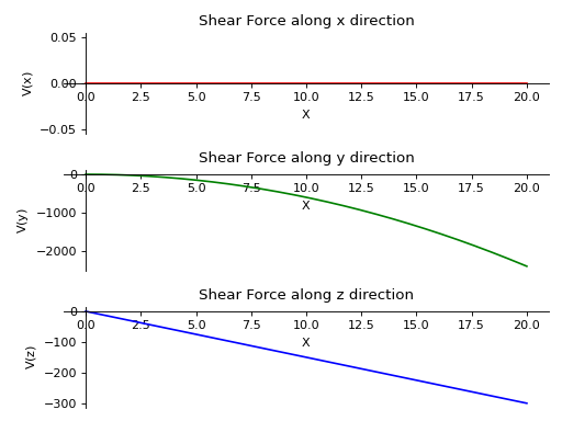
- plot_shear_force(dir='all', subs=None)[源代码]#
Returns a plot for Shear force along all three directions present in the Beam object.
- 参数:
dir : string (default
Direction along which shear force plot is required. If no direction is specified, all plots are displayed.
subs :字典
Python字典,包含作为键的符号及其相应的值。
实例
There is a beam of length 20 meters. It is supported by rollers at both of its ends. A linear load having slope equal to 12 is applied along y-axis. A constant distributed load of magnitude 15 N is applied from start till its end along z-axis.
>>> from sympy.physics.continuum_mechanics.beam import Beam3D
>>> from sympy import symbols
>>> l, E, G, I, A, x = symbols('l, E, G, I, A, x')
>>> b = Beam3D(20, E, G, I, A, x)
>>> b.apply_load(15, start=0, order=0, dir="z")
>>> b.apply_load(12*x, start=0, order=0, dir="y")
>>> b.bc_deflection = [(0, [0, 0, 0]), (20, [0, 0, 0])]
>>> R1, R2, R3, R4 = symbols('R1, R2, R3, R4')
>>> b.apply_load(R1, start=0, order=-1, dir="z")
>>> b.apply_load(R2, start=20, order=-1, dir="z")
>>> b.apply_load(R3, start=0, order=-1, dir="y")
>>> b.apply_load(R4, start=20, order=-1, dir="y")
>>> b.solve_for_reaction_loads(R1, R2, R3, R4)
>>> b.plot_shear_force()
PlotGrid object containing:
Plot[0]:Plot object containing:
[0]: cartesian line: 0 for x over (0.0, 20.0)
Plot[1]:Plot object containing:
[0]: cartesian line: -6*x**2 for x over (0.0, 20.0)
Plot[2]:Plot object containing:
[0]: cartesian line: -15*x for x over (0.0, 20.0)

- plot_shear_stress(dir='all', subs=None)[源代码]#
Returns a plot for Shear Stress along all three directions present in the Beam object.
- 参数:
dir : string (default
Direction along which shear stress plot is required. If no direction is specified, all plots are displayed.
subs :字典
Python字典,包含作为键的符号及其相应的值。
实例
There is a beam of length 20 meters and area of cross section 2 square meters. It is supported by rollers at both of its ends. A linear load having slope equal to 12 is applied along y-axis. A constant distributed load of magnitude 15 N is applied from start till its end along z-axis.
>>> from sympy.physics.continuum_mechanics.beam import Beam3D
>>> from sympy import symbols
>>> l, E, G, I, A, x = symbols('l, E, G, I, A, x')
>>> b = Beam3D(20, E, G, I, 2, x)
>>> b.apply_load(15, start=0, order=0, dir="z")
>>> b.apply_load(12*x, start=0, order=0, dir="y")
>>> b.bc_deflection = [(0, [0, 0, 0]), (20, [0, 0, 0])]
>>> R1, R2, R3, R4 = symbols('R1, R2, R3, R4')
>>> b.apply_load(R1, start=0, order=-1, dir="z")
>>> b.apply_load(R2, start=20, order=-1, dir="z")
>>> b.apply_load(R3, start=0, order=-1, dir="y")
>>> b.apply_load(R4, start=20, order=-1, dir="y")
>>> b.solve_for_reaction_loads(R1, R2, R3, R4)
>>> b.plot_shear_stress()
PlotGrid object containing:
Plot[0]:Plot object containing:
[0]: cartesian line: 0 for x over (0.0, 20.0)
Plot[1]:Plot object containing:
[0]: cartesian line: -3*x**2 for x over (0.0, 20.0)
Plot[2]:Plot object containing:
[0]: cartesian line: -15*x/2 for x over (0.0, 20.0)

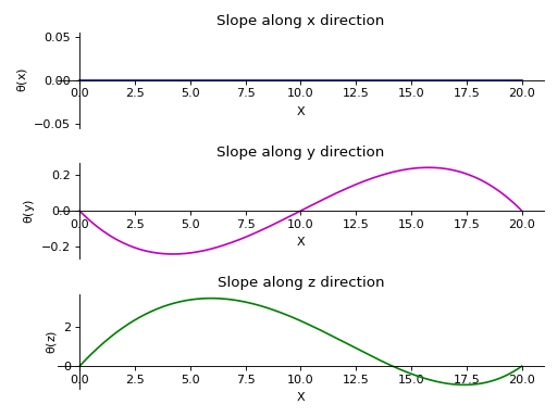
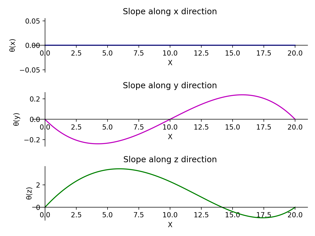
- plot_slope(dir='all', subs=None)[源代码]#
Returns a plot for Slope along all three directions present in the Beam object.
- 参数:
dir : string (default
Direction along which Slope plot is required. If no direction is specified, all plots are displayed.
subs :字典
Python dictionary containing Symbols as keys and their corresponding values.
实例
There is a beam of length 20 meters. It is supported by rollers at both of its ends. A linear load having slope equal to 12 is applied along y-axis. A constant distributed load of magnitude 15 N is applied from start till its end along z-axis.
>>> from sympy.physics.continuum_mechanics.beam import Beam3D
>>> from sympy import symbols
>>> l, E, G, I, A, x = symbols('l, E, G, I, A, x')
>>> b = Beam3D(20, 40, 21, 100, 25, x)
>>> b.apply_load(15, start=0, order=0, dir="z")
>>> b.apply_load(12*x, start=0, order=0, dir="y")
>>> b.bc_deflection = [(0, [0, 0, 0]), (20, [0, 0, 0])]
>>> R1, R2, R3, R4 = symbols('R1, R2, R3, R4')
>>> b.apply_load(R1, start=0, order=-1, dir="z")
>>> b.apply_load(R2, start=20, order=-1, dir="z")
>>> b.apply_load(R3, start=0, order=-1, dir="y")
>>> b.apply_load(R4, start=20, order=-1, dir="y")
>>> b.solve_for_reaction_loads(R1, R2, R3, R4)
>>> b.solve_slope_deflection()
>>> b.plot_slope()
PlotGrid object containing:
Plot[0]:Plot object containing:
[0]: cartesian line: 0 for x over (0.0, 20.0)
Plot[1]:Plot object containing:
[0]: cartesian line: -x**3/1600 + 3*x**2/160 - x/8 for x over (0.0, 20.0)
Plot[2]:Plot object containing:
[0]: cartesian line: x**4/8000 - 19*x**2/172 + 52*x/43 for x over (0.0, 20.0)

- polar_moment()[源代码]#
返回梁绕X轴相对于质心的面积极矩。
实例
>>> from sympy.physics.continuum_mechanics.beam import Beam3D
>>> from sympy import symbols
>>> l, E, G, I, A = symbols('l, E, G, I, A')
>>> b = Beam3D(l, E, G, I, A)
>>> b.polar_moment()
2*I
>>> I1 = [9, 15]
>>> b = Beam3D(l, E, G, I1, A)
>>> b.polar_moment()
24
- property second_moment#
梁面积的二阶矩。
- property shear_modulus#
梁的杨氏模量。
- solve_for_reaction_loads(*reaction)[源代码]#
求解反作用力。
实例
有一根30米长的横梁。它的末端由滚轴支撑。沿y轴从头到尾施加8N的恒定分布载荷。沿z轴施加另一个坡度等于9的线性荷载。
>>> from sympy.physics.continuum_mechanics.beam import Beam3D
>>> from sympy import symbols
>>> l, E, G, I, A, x = symbols('l, E, G, I, A, x')
>>> b = Beam3D(30, E, G, I, A, x)
>>> b.apply_load(8, start=0, order=0, dir="y")
>>> b.apply_load(9*x, start=0, order=0, dir="z")
>>> b.bc_deflection = [(0, [0, 0, 0]), (30, [0, 0, 0])]
>>> R1, R2, R3, R4 = symbols('R1, R2, R3, R4')
>>> b.apply_load(R1, start=0, order=-1, dir="y")
>>> b.apply_load(R2, start=30, order=-1, dir="y")
>>> b.apply_load(R3, start=0, order=-1, dir="z")
>>> b.apply_load(R4, start=30, order=-1, dir="z")
>>> b.solve_for_reaction_loads(R1, R2, R3, R4)
>>> b.reaction_loads
{R1: -120, R2: -120, R3: -1350, R4: -2700}
- solve_for_torsion()[源代码]#
Solves for the angular deflection due to the torsional effects of moments being applied in the x-direction i.e. out of or into the beam.
Here, a positive torque means the direction of the torque is positive i.e. out of the beam along the beam-axis. Likewise, a negative torque signifies a torque into the beam cross-section.
实例
>>> from sympy.physics.continuum_mechanics.beam import Beam3D
>>> from sympy import symbols
>>> l, E, G, I, A, x = symbols('l, E, G, I, A, x')
>>> b = Beam3D(20, E, G, I, A, x)
>>> b.apply_moment_load(4, 4, -2, dir='x')
>>> b.apply_moment_load(4, 8, -2, dir='x')
>>> b.apply_moment_load(4, 8, -2, dir='x')
>>> b.solve_for_torsion()
>>> b.angular_deflection().subs(x, 3)
18/(G*I)