

物理模型#
这些模型都是物理驱动的,通常作为物理问题的解决方案。这与那些通常作为数学问题解决方案的数学动机形成鲜明对比。
BlackBody#
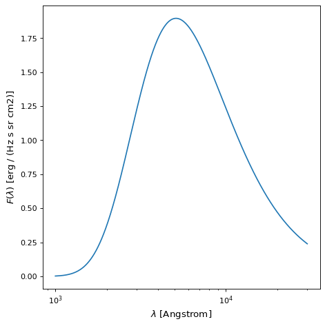
这个 BlackBody 模型提供了一个用于 Planck's Law . 黑体函数是
在哪里? \(\nu\) 是频率, \(T\) 是温度, \(A\) 是比例因子, \(h\) 普朗克常数, \(c\) 是光速 \(k\) 玻尔兹曼常数。
模型的两个参数:比例因子 scale (A) 以及绝对温度 temperature (T) 一。如果 scale 因子没有单位,则结果是以光谱辐射度为单位,特别是ergs/(cm^2 Hz s sr)。如果 scale 因子与光谱辐射度单位一起传递,则结果以这些单位表示(例如,ergs/(cm^2 A s sr)或MJy/sr)。设置 scale 单位为ergs/(cm^2 A s sr)的因子将使普朗克函数为 \(B_\lambda\) . 温度可以通过任何支持的温度单位作为一个量传递。
下面是一个温度为10000 K,标度为1的黑体的示例图。小数位数为1表示普朗克函数,返回的默认单位没有缩放 BlackBody .
import numpy as np
import matplotlib.pyplot as plt

from astropy.modeling.models import BlackBody
import astropy.units as u

wavelengths = np.logspace(np.log10(1000), np.log10(3e4), num=1000) * u.AA

# blackbody parameters
temperature = 10000 * u.K

# BlackBody provides the results in ergs/(cm^2 Hz s sr) when scale has no units
bb = BlackBody(temperature=temperature, scale=10000.0)
bb_result = bb(wavelengths)

fig, ax = plt.subplots(layout='tight')
ax.plot(wavelengths, bb_result, '-')

ax.set(
    xscale="log",
    xlabel=fr"$\lambda$ [{wavelengths.unit}]",
    ylabel=fr"$F(\lambda)$ [{bb_result.unit}]",
)

plt.show()

这个 bolometric_flux() 成员函数使用 \(\sigma T^4/\pi\) 在哪里? \(\sigma\) 是Stefan Boltzmann常数。
这个 lambda_max() 和 nu_max() 成员函数给出了 \(B_\lambda\) 和 \(B_\nu\) ,分别使用 Wien's Law .
德鲁德1D#
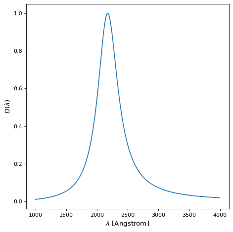
这个 Drude1D 模型提供了一个材料中电子行为的模型(参见 Drude Model ). 就像 Lorentz1D 模型,德鲁德模型的翅膀比 Gaussian1D 模型。德鲁德剖面已用于模拟尘埃特征,包括2175埃消光特征和中红外芳香族/PAH特征。德鲁德在 \(x\) 是
在哪里? \(A\) 是振幅, \(f\) 是最大宽度的一半,以及 \(x_0\) 是中心波长。Drude1D模型的示例 \(x_0 = 2175\) 埃和 \(f = 400\) 埃如下所示。
import numpy as np
import matplotlib.pyplot as plt

from astropy.modeling.models import Drude1D
import astropy.units as u

wavelengths = np.linspace(1000, 4000, num=1000) * u.AA

# Parameters and model
mod = Drude1D(amplitude=1.0, x_0=2175. * u.AA, fwhm=400. * u.AA)
mod_result = mod(wavelengths)

fig, ax = plt.subplots(layout="tight")
ax.plot(wavelengths, mod_result, '-')

ax.set(xlabel=fr"$\lambda$ [{wavelengths.unit}]", ylabel=r"$D(\lambda)$")

plt.show()

NFW#
这个 NFW 该模型计算了一维纳瓦罗-弗伦克-怀特轮廓。NFW剖面中的暗物质密度由以下公式给出:
在哪里? \(\rho_{{c}}\) 是轮廓红移时宇宙的临界密度, \(\delta_c\) 是过密度,以及 \(r_s\) 是轮廓的缩放半径。
该模型依赖于三个参数:
mass:剖面的质量(如果未提供单位,则以太阳质量为单位)
concentration:剖面浓度
redshift:外形的红移
以及两个可选的初始化变量:
massfactor:指定过敏感类型和因子的元组或字符串(默认值为“临界”,200))
cosmo:用于密度计算的宇宙学(默认默认值_宇宙学)
备注
评估前需要初始化NFW轮廓物体(以便设置质量过密度和宇宙学)。
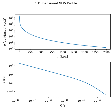
- 具有以下参数的NFW剖面图示例如下所示:
mass= \(2.0 x 10^{15} M_{sun}\)concentration=8.5redshift=0.63
第一张图是NFW剖面密度与半径的函数关系。第二个绘图分别显示由NFW比例密度和比例半径规范化的剖面密度和半径。“缩放密度”(scale density)和“缩放半径”(scale radius)可用作属性 rho_s 和 r_s ,可通过 r_virial .
import numpy as np
import matplotlib.pyplot as plt
from astropy.modeling.models import NFW
import astropy.units as u
from astropy import cosmology

# NFW Parameters
mass = u.Quantity(2.0E15, u.M_sun)
concentration = 8.5
redshift = 0.63
cosmo = cosmology.Planck15
massfactor = ("critical", 200)

# Create NFW Object
n = NFW(mass=mass, concentration=concentration, redshift=redshift, cosmo=cosmo,
        massfactor=massfactor)

# Radial distribution for plotting
radii = range(1,2001,10) * u.kpc

# Radial NFW density distribution
n_result = n(radii)

# Plot creation
fig, axs = plt.subplots(nrows=2)
fig.suptitle('1 Dimensional NFW Profile')

# Density profile subplot
axs[0].plot(radii, n_result, '-')
axs[0].set(
    yscale='log',
    xlabel=fr"$r$ [{radii.unit}]",
    ylabel=fr"$\rho$ [{n_result.unit}]",
)

# Create scaled density / scaled radius subplot
# NFW Object
n = NFW(mass=mass, concentration=concentration, redshift=redshift, cosmo=cosmo,
        massfactor=massfactor)

# Radial distribution for plotting
radii = np.logspace(np.log10(1e-5), np.log10(2), num=1000) * u.Mpc
n_result = n(radii)

# Scaled density / scaled radius subplot
axs[1].plot(radii / n.radius_s, n_result / n.density_s, '-')
axs[1].set(
    xscale='log',
    yscale='log',
    xlabel=r"$r / r_s$",
    ylabel=r"$\rho / \rho_s$",
)

# Display plot
fig.tight_layout(rect=[0, 0.03, 1, 0.95])
plt.show()

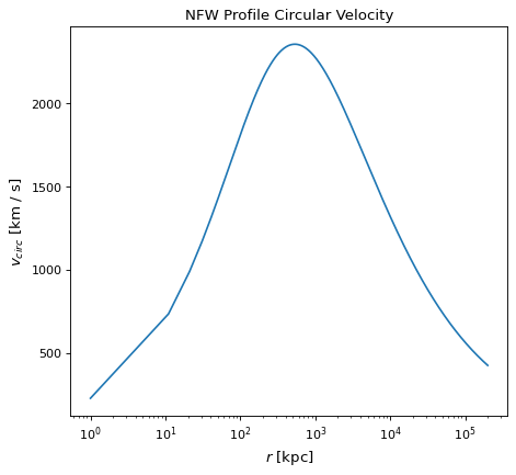
这个 circular_velocity() 构件提供每个位置的圆速度 r 通过方程式:
其中x是比率 r :数学:/r_{vir}。圆速度是以公里/秒为单位提供的。
具有以下参数的NFW剖面的圆速度示例图如下所示:
mass= \(2.0 x 10^{15} M_{sun}\)
concentration=8.5
redshift=0.63
“最大圆速度”和“最大圆速度半径”作为属性可用 v_max 和 r_max .
import matplotlib.pyplot as plt
from astropy.modeling.models import NFW
import astropy.units as u
from astropy import cosmology

# NFW Parameters
mass = u.Quantity(2.0E15, u.M_sun)
concentration = 8.5
redshift = 0.63
cosmo = cosmology.Planck15
massfactor = ("critical", 200)

# Create NFW Object
n = NFW(mass=mass, concentration=concentration, redshift=redshift, cosmo=cosmo,
        massfactor=massfactor)

# Radial distribution for plotting
radii = range(1,200001,10) * u.kpc

# NFW circular velocity distribution
n_result = n.circular_velocity(radii)

# Plot creation
fig,ax = plt.subplots()
ax.set_title('NFW Profile Circular Velocity')
ax.plot(radii, n_result, '-')
ax.set_xscale('log')
ax.set_xlabel(fr"$r$ [{radii.unit}]")
ax.set_ylabel(r"$v_{circ}$" + f" [{n_result.unit}]")

# Display plot
plt.tight_layout(rect=[0, 0.03, 1, 0.95])
plt.show()

宇宙学#
的实例 Cosmology 类(和子类)包括|Cosmology.to_Format|,这是一种将Cosmology转换为另一个Python对象的方法。具体地说,任何红移方法都可以转换为 FittableModel 使用参数实例化 format="astropy.model" 。在转换过程中,每个 Cosmology Parameter 被转换为 astropy.modeling.Model Parameter ,而红移方法则成为模型的 __call__ / evaluate 方法。这意味着宇宙学现在可以用数据来拟合了!
>>> from astropy.cosmology import Planck18
>>> model = Planck18.to_format(format="astropy.model", method="lookback_time")
>>> model
<FlatLambdaCDMCosmologyLookbackTimeModel(H0=67.66 km / (Mpc s), Om0=0.30966,
    Tcmb0=2.7255 K, Neff=3.046, m_nu=[0.  , 0.  , 0.06] eV, Ob0=0.04897,
    name='Planck18')>
完成后,例如试衣,可以将模型转换回 Cosmology 使用|Cosmology.from_Format|。
>>> from astropy.cosmology import Cosmology
>>> cosmo = Cosmology.from_format(model, format="astropy.model")
>>> cosmo == Planck18
True