
不确定性和分布 (astropy.uncertainty )#
介绍#
备注
这个子包仍在开发中。
astropy 提供了一个 Distribution 对象表示统计分布的形式,该形式充当 Quantity 对象或常规 numpy.ndarray . 以这种方式使用, Distribution 以额外计算为代价提供不确定性传播。例如,它还可以更一般地表示蒙特卡罗计算技术中的抽样分布。
这个特性的核心对象是 Distribution . 目前,所有这些分布都是蒙特卡罗抽样的。虽然这意味着每个分布可能需要更多的内存,但它允许在保持其相关性结构的同时对分布执行任意复杂的操作。一些特定的良好分布(如正态分布)具有分析形式,最终可能使表示更加紧凑和有效。在未来,这些可能会提供一种相干的不确定性传播机制 NDData . 但是,目前还没有实施。因此,存储不确定性的细节 NDData 对象可以在 N维数据集 (astropy.nddata ) 部分。
入门#
要演示分布的基本用例,请考虑正态分布的不确定性传播问题。假设有两个测量值需要添加,每个测量值都具有正常的不确定度。我们从一些初始导入和设置开始:
>>> import numpy as np
>>> from astropy import units as u
>>> from astropy import uncertainty as unc
>>> rng = np.random.default_rng(12345)  # ensures reproducible example numbers
现在我们创建两个 Distribution 对象来表示我们的分布:
>>> a = unc.normal(1*u.kpc, std=30*u.pc, n_samples=10000)
>>> b = unc.normal(2*u.kpc, std=40*u.pc, n_samples=10000)
对于正态分布,中心应按预期增加,标准差应加入求积。我们可以用 Distribution 算术和属性:
>>> c = a + b
>>> c
<QuantityDistribution [...] kpc with n_samples=10000>
>>> c.pdf_mean()
<Quantity 2.99970555 kpc>
>>> c.pdf_std().to(u.pc)
<Quantity 50.07120457 pc>
事实上,这些都接近预期。虽然对于基本的高斯情况,对于更复杂的分布或算术运算,误差分析变得站不住脚,这似乎是不必要的, Distribution 仍然可以通过:
>>> d = unc.uniform(center=3*u.kpc, width=800*u.pc, n_samples=10000)
>>> e = unc.Distribution(((rng.beta(2,5, 10000)-(2/7))/2 + 3)*u.kpc)
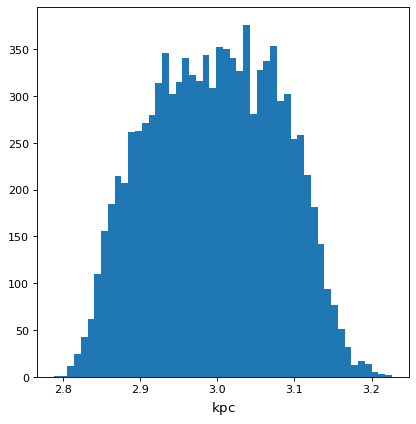
>>> f = (c * d * e) ** (1/3)
>>> f.pdf_mean()
<Quantity 2.99760998 kpc>
>>> f.pdf_std()
<Quantity 0.08308941 kpc>
>>> from matplotlib import pyplot as plt
>>> from astropy.visualization import quantity_support
>>> with quantity_support():
... plt.hist(f.distribution, bins=50)
使用 astropy.uncertainty#
创建分发#
创建分布最直接的方法是使用数组或 Quantity 带着样本 last 尺寸:
>>> import numpy as np
>>> from astropy import units as u
>>> from astropy import uncertainty as unc
>>> rng = np.random.default_rng(123456)  # ensures "random" numbers match examples below
>>> unc.Distribution(rng.poisson(12, (1000)))
NdarrayDistribution([..., 12,...]) with n_samples=1000
>>> pq = rng.poisson([1, 5, 30, 400], (1000, 4)).T * u.ct # note the transpose, required to get the sampling on the *last* axis
>>> distr = unc.Distribution(pq)
>>> distr
<QuantityDistribution [[...],
           [...],
           [...],
           [...]] ct with n_samples=1000>
请注意这两个发行版的区别:第一个发行版是从数组构建的,因此没有 Quantity 像 unit 后者有这些属性。这反映在它们如何与其他对象交互,例如 NdarrayDistribution 不会与 Quantity 包含单位的对象。
对于常用的发行版,helper函数的存在使创建它们更加方便。下面的示例演示了几种创建正态/高斯分布的等效方法:
>>> center = [1, 5, 30, 400]
>>> n_distr = unc.normal(center*u.kpc, std=[0.2, 1.5, 4, 1]*u.kpc, n_samples=1000)
>>> n_distr = unc.normal(center*u.kpc, var=[0.04, 2.25, 16, 1]*u.kpc**2, n_samples=1000)
>>> n_distr = unc.normal(center*u.kpc, ivar=[25, 0.44444444, 0.625, 1]*u.kpc**-2, n_samples=1000)
>>> n_distr.distribution.shape
(4, 1000)
>>> unc.normal(center*u.kpc, std=[0.2, 1.5, 4, 1]*u.kpc, n_samples=100).distribution.shape
(4, 100)
>>> unc.normal(center*u.kpc, std=[0.2, 1.5, 4, 1]*u.kpc, n_samples=20000).distribution.shape
(4, 20000)
此外,泊松和均匀 Distribution 存在创建函数:
>>> unc.poisson(center*u.count, n_samples=1000)
<QuantityDistribution [[...],
             [...],
             [...],
             [...]] ct with n_samples=1000>
>>> uwidth = [10, 20, 10, 55]*u.pc
>>> unc.uniform(center=center*u.kpc, width=uwidth, n_samples=1000)
<QuantityDistribution [[...],
             [...],
             [...],
             [...]] kpc with n_samples=1000>
>>> unc.uniform(lower=center*u.kpc - uwidth/2,  upper=center*u.kpc + uwidth/2, n_samples=1000)
<QuantityDistribution [[...],
             [...],
             [...],
             [...]] kpc with n_samples=1000>
用户可以按照类似的模式自由创建自己的分发类。
使用分布#
这个对象现在的行为很像 Quantity 或 numpy.ndarray 对于除非采样维度以外的所有维度,但具有对采样分布起作用的其他统计操作:
>>> distr.shape
(4,)
>>> distr.size
4
>>> distr.unit
Unit("ct")
>>> distr.n_samples
1000
>>> distr.pdf_mean()
<Quantity [  1.034,   5.026,  29.994, 400.365] ct>
>>> distr.pdf_std()
<Quantity [ 1.04539179,  2.19484031,  5.47776998, 19.87022333] ct>
>>> distr.pdf_var()
<Quantity [  1.092844,   4.817324,  30.005964, 394.825775] ct2>
>>> distr.pdf_median()
<Quantity [   1.,   5.,  30., 400.] ct>
>>> distr.pdf_mad()  # Median absolute deviation
<Quantity [ 1.,  1.,  4., 13.] ct>
>>> distr.pdf_smad()  # Median absolute deviation, rescaled to match std for normal
<Quantity [ 1.48260222,  1.48260222,  5.93040887, 19.27382884] ct>
>>> distr.pdf_percentiles([10, 50, 90])
<Quantity [[  0. ,   2. ,  23. , 375. ],
           [  1. ,   5. ,  30. , 400. ],
           [  2. ,   8. ,  37. , 426.1]] ct>
>>> distr.pdf_percentiles([.1, .5, .9]*u.dimensionless_unscaled)
<Quantity [[  0. ,   2. ,  23. , 375. ],
          [  1. ,   5. ,  30. , 400. ],
          [  2. ,   8. ,  37. , 426.1]] ct>
如果需要,可以从 distribution 属性:
>>> distr.distribution
<Quantity [[  2.,   2.,   0., ...,   1.,   0.,   1.],
           [  3.,   2.,   8., ...,   8.,   3.,   3.],
           [ 31.,  30.,  32., ...,  20.,  34.,  31.],
           [354., 373., 384., ..., 410., 404., 395.]] ct>
>>> distr.distribution.shape
(4, 1000)
A Quantity distribution interacts naturally with non-Distribution
Quantity objects, assuming the Quantity is a Dirac delta distribution:
>>> distr_in_kpc = distr * u.kpc/u.count  # for the sake of round numbers in examples
>>> distrplus = distr_in_kpc + [2000,0,0,500]*u.pc
>>> distrplus.pdf_median()
<Quantity [   3. ,   5. ,  30. , 400.5] kpc>
>>> distrplus.pdf_var()
<Quantity [  1.092844,   4.817324,  30.005964, 394.825775] kpc2>
它在其他分布中也按预期运行(但协方差的讨论见下文):
>>> means = [2000, 0, 0, 500]
>>> sigmas = [1000, .01, 3000, 10]
>>> another_distr = unc.Distribution((rng.normal(means, sigmas, (1000,4))).T * u.pc)
>>> combined_distr = distr_in_kpc + another_distr
>>> combined_distr.pdf_median()
<Quantity [  2.81374275,   4.99999631,  29.7150889 , 400.49576691] kpc>
>>> combined_distr.pdf_var()
<Quantity [  2.15512118,   4.817324  ,  39.0614616 , 394.82969655] kpc2>
分布协方差与离散抽样效应#
分布的主要应用之一是不确定性传播,这就要求正确处理协方差。这在montecarlo采样方法中很自然 Distribution 类,只要适当注意采样误差。
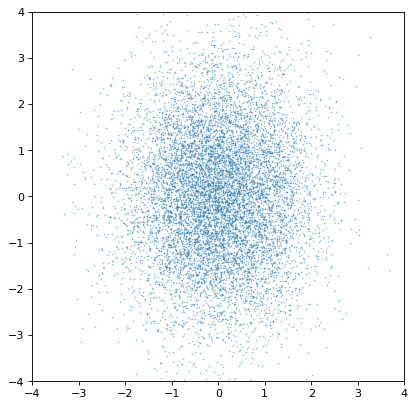
从一个基本的例子开始,两个不相关的分布应该产生一个不相关的联合分布图:
>>> import numpy as np
>>> from astropy import units as u
>>> from astropy import uncertainty as unc
>>> from matplotlib import pyplot as plt
>>> n1 = unc.normal(center=0., std=1, n_samples=10000)
>>> n2 = unc.normal(center=0., std=2, n_samples=10000)
>>> plt.scatter(n1.distribution, n2.distribution, s=2, lw=0, alpha=.5)
>>> plt.xlim(-4, 4)
>>> plt.ylim(-4, 4)
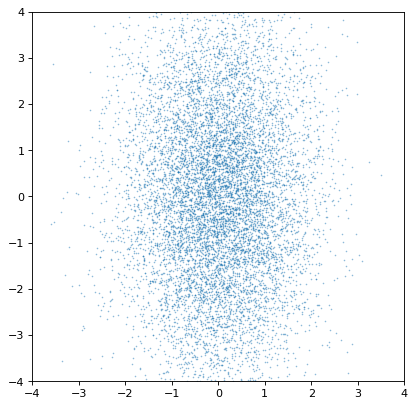
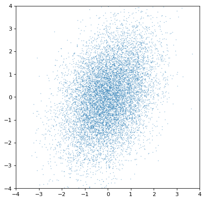
事实上,这些分布是独立的。如果我们相反地构造一对协变高斯数,它会很明显:
>>> rng = np.random.default_rng(357)
>>> ncov = rng.multivariate_normal([0, 0], [[1, .5], [.5, 2]], size=10000)
>>> n1 = unc.Distribution(ncov[:, 0])
>>> n2 = unc.Distribution(ncov[:, 1])
>>> plt.scatter(n1.distribution, n2.distribution, s=2, lw=0, alpha=.5)
>>> plt.xlim(-4, 4)
>>> plt.ylim(-4, 4)

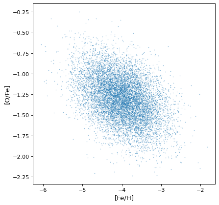
最重要的是,适当的相关结构被保存或通过适当的算术运算生成。例如,如果轴不是独立的,则不相关正态分布的比率将获得协方差,如在假设的恒星集合中对铁、氢和氧丰度的模拟:
>>> fe_abund = unc.normal(center=-2, std=.25, n_samples=10000)
>>> o_abund = unc.normal(center=-6., std=.5, n_samples=10000)
>>> h_abund = unc.normal(center=-0.7, std=.1, n_samples=10000)
>>> feh = fe_abund - h_abund
>>> ofe = o_abund - fe_abund
>>> plt.scatter(ofe.distribution, feh.distribution, s=2, lw=0, alpha=.5)
>>> plt.xlabel('[Fe/H]')
>>> plt.ylabel('[O/Fe]')

这表明,相关性自然地产生于变量,但无需明确解释:采样过程自然地恢复存在的相关性。
然而,一个重要的警告是,只有当采样轴逐样本完全匹配时,协方差才会被保留。如果不是,则所有协方差信息(静默)丢失:
>>> n2_wrong = unc.Distribution(ncov[::-1, 1])  #reverse the sampling axis order
>>> plt.scatter(n1.distribution, n2_wrong.distribution, s=2, lw=0, alpha=.5)
>>> plt.xlim(-4, 4)
>>> plt.ylim(-4, 4)
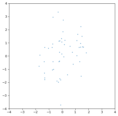
此外,抽样不足的分布可能给出较差的估计或隐藏相关性。下面的示例与上面的协变高斯示例相同,但采样数减少了200倍:
>>> ncov = rng.multivariate_normal([0, 0], [[1, .5], [.5, 2]], size=50)
>>> n1 = unc.Distribution(ncov[:, 0])
>>> n2 = unc.Distribution(ncov[:, 1])
>>> plt.scatter(n1.distribution, n2.distribution, s=5, lw=0)
>>> plt.xlim(-4, 4)
>>> plt.ylim(-4, 4)
>>> np.cov(n1.distribution, n2.distribution)
array([[0.95534365, 0.35220031],
       [0.35220031, 1.99511743]])

协方差结构肉眼看不太明显,这反映在输入和输出协方差矩阵之间的显著差异上。一般来说,这是使用抽样分布的内在权衡:样本数量越少,计算效率越高,但在任何相关数量中都会导致更大的不确定性。这些都是有秩序的 \(\sqrt{{n_{{\rm samples}}}}\) 但这取决于所讨论的分布的复杂性。
参考/API#
不确定性包裹#
此子程序包包含用于创建工作原理类似于 Quantity 或数组对象,但会传播不确定性。
功能#
|
创建高斯/正态分布。 |
|
创建泊松分布。 |
|
从上下限创建一个统一的分布。 |
Classes#
|
具有相关不确定性分布的标量值或数组值。 |