

天文坐标系 (astropy.coordinates )#
介绍#
这个 coordinates 该包提供了表示各种天体/空间坐标及其速度分量的类,以及以统一方式在公共坐标系之间转换的工具。
入门#
开始使用的最佳方式 coordinates 就是使用 SkyCoord 班级。 SkyCoord 通过传入具有指定单位和坐标框架的位置(和可选速度)来实例化对象。天空位置通常作为 Quantity 对象,并且使用字符串名称指定框架。
要创建 SkyCoord 对象来表示ICRS(右升角 [RA] 、赤纬 [Dec] )天空位置::
>>> from astropy import units as u
>>> from astropy.coordinates import SkyCoord
>>> c = SkyCoord(ra=10.625*u.degree, dec=41.2*u.degree, frame='icrs')
的初始值设定项 SkyCoord 非常灵活,并支持以多种方便的格式提供的输入。以下初始化坐标的方法都等同于上面的方法:
>>> c = SkyCoord(10.625, 41.2, frame='icrs', unit='deg')
>>> c = SkyCoord('00h42m30s', '+41d12m00s', frame='icrs')
>>> c = SkyCoord('00h42.5m', '+41d12m')
>>> c = SkyCoord('00 42 30 +41 12 00', unit=(u.hourangle, u.deg))
>>> c = SkyCoord('00:42.5 +41:12', unit=(u.hourangle, u.deg))
>>> c
<SkyCoord (ICRS): (ra, dec) in deg
    (10.625, 41.2)>
上面的示例说明了创建坐标对象时要遵循的一些规则:
坐标值可以作为未命名的位置参数或通过关键字参数提供,例如
ra和dec或l和b(取决于框架)。坐标系
frame关键字是可选的,因为它默认为ICRS.必须为所有组件指定角度单位,或者传入
Quantity对象(例如,10.5*u.degree),通过将它们包含在值中(例如。,'+41d12m00s'),或通过unit关键字。
SkyCoord 以及所有其他 coordinates 对象还支持数组坐标。这些坐标的工作方式与单值坐标相同,但它们在单个对象中存储多个坐标。当您要将相同的操作应用于许多不同的坐标时(比方说,从目录中),这是一个比列表 SkyCoord 对象,因为它将是 much 比将运算分别应用于 SkyCoord 在一个 for 循环播放。就像潜在的 ndarray 包含数据的实例, SkyCoord 可以对对象进行切片、整形等操作,并且可以与如下功能一起使用 numpy.moveaxis 等,它们会影响形状:
>>> import numpy as np
>>> c = SkyCoord(ra=[10, 11, 12, 13]*u.degree, dec=[41, -5, 42, 0]*u.degree)
>>> c
<SkyCoord (ICRS): (ra, dec) in deg
    [(10., 41.), (11., -5.), (12., 42.), (13.,  0.)]>
>>> c[1]
<SkyCoord (ICRS): (ra, dec) in deg
    (11., -5.)>
>>> c.reshape(2, 2)
<SkyCoord (ICRS): (ra, dec) in deg
    [[(10., 41.), (11., -5.)],
     [(12., 42.), (13.,  0.)]]>
>>> np.roll(c, 1)
<SkyCoord (ICRS): (ra, dec) in deg
    [(13.,  0.), (10., 41.), (11., -5.), (12., 42.)]>
协调访问#
一旦你有了一个坐标对象,你就可以访问这个坐标的组件(例如,RA,Dec)来获得完整坐标的字符串表示。
组件值是使用(通常是小写)命名属性访问的,这些属性依赖于坐标系(例如,ICRS、Galactic等)。默认情况下,坐标组件名称为 ra 和 dec ::
>>> c = SkyCoord(ra=10.68458*u.degree, dec=41.26917*u.degree)
>>> c.ra
<Longitude 10.68458 deg>
>>> c.ra.hour
np.float64(0.7123053333333335)
>>> c.ra.hms
hms_tuple(h=np.float64(0.0), m=np.float64(42.0), s=np.float64(44.299200000000525))
>>> c.dec
<Latitude 41.26917 deg>
>>> c.dec.degree
np.float64(41.26917)
>>> c.dec.radian
np.float64(0.7202828960652683)
可以使用 to_string() 方法:
>>> c = SkyCoord(ra=10.68458*u.degree, dec=41.26917*u.degree)
>>> c.to_string('decimal')
'10.6846 41.2692'
>>> c.to_string('dms')
'10d41m04.488s 41d16m09.012s'
>>> c.to_string('hmsdms')
'00h42m44.2992s +41d16m09.012s'
有关更多信息,请参见 使用角度 .
变换#
转换到新坐标系的一种方便方法是访问适当命名的属性。
以获得 Galactic 帧使用:
>>> c_icrs = SkyCoord(ra=10.68458*u.degree, dec=41.26917*u.degree, frame='icrs')
>>> c_icrs.galactic
<SkyCoord (Galactic): (l, b) in deg
    (121.17424181, -21.57288557)>
为了获得更多的控制,可以使用 transform_to 方法,它接受框架名称、框架类或框架实例:
>>> c_fk5 = c_icrs.transform_to('fk5')  # c_icrs.fk5 does the same thing
>>> c_fk5
<SkyCoord (FK5: equinox=J2000.000): (ra, dec) in deg
    (10.68459154, 41.26917146)>

>>> from astropy.coordinates import FK5
>>> c_fk5.transform_to(FK5(equinox='J1975'))  # precess to a different equinox
<SkyCoord (FK5: equinox=J1975.000): (ra, dec) in deg
    (10.34209135, 41.13232112)>
这种形式的 transform_to 还可以将天体坐标转换为 AltAz 坐标,允许使用 SkyCoord 作为计划观测的工具。有关这方面的更完整的示例,请参见 确定和绘制天体的高度/方位角 。
一些坐标系,例如 AltAz 在转换到/从其他帧转换时需要地球自转信息(UT1-UTC偏移量和/或极轴运动)。这些地球自转值在需要时自动从国际地球自转和参考系统(IERS)服务下载。看到了吗 IERS数据访问 (astropy.utils.iers ) 有关此过程的详细信息。
表现#
到目前为止,我们在所有示例中都使用了球面坐标表示法,这是内置框架的默认设置。通常,使用不同的表示(例如笛卡尔表示或柱面表示)来初始化或使用坐标是很方便的。这可以通过设置 representation_type 对于任何一种 SkyCoord 对象或低级框架坐标对象。
要使用不同的表示法(如笛卡尔坐标或圆柱坐标)初始化坐标或使用坐标,请执行以下操作:
>>> c = SkyCoord(x=1, y=2, z=3, unit='kpc', representation_type='cartesian')
>>> c
<SkyCoord (ICRS): (x, y, z) in kpc
    (1., 2., 3.)>
>>> c.x, c.y, c.z
(<Quantity 1. kpc>, <Quantity 2. kpc>, <Quantity 3. kpc>)

>>> c.representation_type = 'cylindrical'
>>> c
<SkyCoord (ICRS): (rho, phi, z) in (kpc, deg, kpc)
    (2.23606798, 63.43494882, 3.)>
有关所有详细信息,请参见 陈述 .
距离#
SkyCoord 并且各个框架类还支持指定距框架原点的距离。原点取决于特定的坐标系;例如,可以是以地球为中心,以太阳系重心为中心,等等。
两个角度和一个距离指定三维空间中的唯一点,这也允许将坐标转换为笛卡尔表示:
>>> c = SkyCoord(ra=10.68458*u.degree, dec=41.26917*u.degree, distance=770*u.kpc)
>>> c.cartesian.x
<Quantity 568.71286542 kpc>
>>> c.cartesian.y
<Quantity 107.3008974 kpc>
>>> c.cartesian.z
<Quantity 507.88994292 kpc>
在分配了距离后, SkyCoord 方便的方法更强大,因为它们可以利用3D信息。例如,要计算空间中两点之间的物理三维间隔:
>>> c1 = SkyCoord(ra=10*u.degree, dec=9*u.degree, distance=10*u.pc, frame='icrs')
>>> c2 = SkyCoord(ra=11*u.degree, dec=10*u.degree, distance=11.5*u.pc, frame='icrs')
>>> c1.separation_3d(c2)
<Distance 1.52286024 pc>
方便方法#
SkyCoord 定义了许多方便的方法,例如,支持计算两个坐标之间的天空(即角度)和3D分隔。
要计算两个坐标之间的天空和三维距离:
>>> c1 = SkyCoord(ra=10*u.degree, dec=9*u.degree, frame='icrs')
>>> c2 = SkyCoord(ra=11*u.degree, dec=10*u.degree, frame='fk5')
>>> c1.separation(c2)  # Differing frames handled correctly
<Angle 1.40453359 deg>
或交叉匹配目录坐标(详见 匹配目录 ):
>>> target_c = SkyCoord(ra=10*u.degree, dec=9*u.degree, frame='icrs')
>>> # read in coordinates from a catalog...
>>> catalog_c = ...
>>> idx, sep, _ = target_c.match_to_catalog_sky(catalog_c)
这个 astropy.coordinates sub-package also provides a quick way to get coordinates for named objects, assuming you have an active internet connection. The from_name method of SkyCoord uses Sesame 检索特定命名对象的坐标。
要检索特定命名对象的坐标:
>>> SkyCoord.from_name("PSR J1012+5307")
<SkyCoord (ICRS): (ra, dec) in deg
    (153.1393271, 53.117343)>
在某些情况下,坐标嵌入到对象的目录名中。对于这样的对象名, from_name 如果给定 parse=True 选项。对于慢速连接,这可能比针对相同对象名的sesame查询快得多。但是,值得注意的是,以这种方式提取的坐标可能与数据库坐标相差几分秒,因此只有在坐标不需要亚弧秒精度的情况下才使用此选项:
>>> SkyCoord.from_name("CRTS SSS100805 J194428-420209", parse=True)
<SkyCoord (ICRS): (ra, dec) in deg
    (296.11666667, -42.03583333)>
对于地球上的站点(主要是天文台), astropy.coordinates 提供了一种快速获取 EarthLocation -- of_site() 类方法:
>>> from astropy.coordinates import EarthLocation
>>> apo = EarthLocation.of_site('Apache Point Observatory')
>>> apo
<EarthLocation (-1463969.30185172, -5166673.34223433, 3434985.71204565) m>
要查看可用的站点名称列表,请使用 get_site_names() **
>>> EarthLocation.get_site_names()
['ALMA', 'AO', 'ARCA', ...]
Both of_site() and
get_site_names(),
astropy.coordinates attempt to access the site registry from the
astropy-data repository and will
save the registry in the user's local cache (see 可下载数据管理 (astropy.utils.data )). If
there is no local cache and Internet connection is not available, a built-in
list (consisting of only the Greenwich Royal Observatory as an example case) is
loaded. The cached version of the site registry is not updated automatically,
but the latest version may be downloaded using the refresh_cache=True
option of these methods. If you would like a site to be added to the registry,
issue a pull request to the astropy-data repository.
对于任意的地球地址(例如,不是观测站),使用 of_address() 类方法来检索纬度和经度。这适用于完全指定的地址、位置名称、城市名称等:
>>> EarthLocation.of_address('1002 Holy Grail Court, St. Louis, MO')
<EarthLocation (-26769.86528679, -4997007.71191864, 3950273.57633915) m>
默认情况下, OpenStreetMap Nominatim service 是使用的,但通过提供 Google Geocoding API key 与 google_api_key 论点:可以使用谷歌地图来替代。除了经度和纬度之外,还可以查询该位置的高度,但只能使用Google查询:
>>> EarthLocation.of_address("Cape Town", get_height=True)
Traceback (most recent call last):
  ...
ValueError: Currently, `get_height` only works when using the Google
geocoding API...
备注
from_name() , of_site() ,以及 of_address() 都是为了方便,而不是为了准确。如果需要对象的准确坐标,则应找到适当的引用并手动输入坐标,或使用更多专用功能,如 astroquery 或 astroplan 关联套餐。
还要注意的是,这些方法从互联网上检索数据来确定天文或地理坐标。在线数据可能会更新,因此如果您需要保证您的脚本长期可重现,请参阅 访问远程资源的方法的使用提示/建议 一节。
可以组合此功能来执行更复杂的任务,如计算径向速度观测值的重心改正(也是支持的高级 SkyCoord 方法-请参阅 径向速度修正 ):
>>> from astropy.time import Time
>>> obstime = Time('2017-2-14')
>>> target = SkyCoord.from_name('M31')
>>> keck = EarthLocation.of_site('Keck')
>>> target.radial_velocity_correction(obstime=obstime, location=keck).to('km/s')
<Quantity -22.359784554780255 km / s>
而当 astropy.coordinates 本身不支持将地球位置转换为时区,可以从任何 EarthLocation object, which could then be passed to any third-party package that supports timezone solving, such as timezonefinder ,在这种情况下,您可能需要将它们的 .degree 属性。
然后,生成的时区名称可以与任何支持时区定义的包一起使用,例如 zoneinfo :
>>> import datetime
>>> from zoneinfo import ZoneInfo
>>> tz = ZoneInfo('America/Phoenix')
>>> dt = datetime.datetime(2021, 4, 12, 20, 0, 0, tzinfo=tz)
速度(固有运动和径向速度)#
除了位置坐标之外, coordinates 支持存储和转换速度。这些都可以通过较低级别的 coordinate frame classes 、和VIA SkyCoord 对象::
>>> sc = SkyCoord(1*u.deg, 2*u.deg, radial_velocity=20*u.km/u.s)
>>> sc
<SkyCoord (ICRS): (ra, dec) in deg
    (1., 2.)
 (radial_velocity) in km / s
    (20.,)>
有关速度支持(和限制)的更多详细信息,请参见 在天文坐标系中处理速度 页。
口罩#
有时您可能拥有有关对象的不完整信息,例如,有些人有距离,而另一些人则没有。 coordinates 支持将掩码用于此类目的,使用 Masked 类别::
>>> from astropy.utils.masked import Masked
>>> distance = Masked([0.1, np.nan]*u.kpc, mask=[False, True])
>>> sc = SkyCoord([1., 2.]*u.hourangle, [3., 4.]*u.deg, distance=distance)
>>> sc
<SkyCoord (ICRS): (ra, dec, distance) in (deg, deg, kpc)
    [(15., 3., 0.1), (30., 4., ———)]>
面具如您所期望的那样传播::
>>> sc.separation(sc[0])
<MaskedAngle [ 0.        , 15.00502838] deg>
>>> sc.separation_3d(sc[0])
<MaskedDistance [ 0., ———] kpc>
>>> gcrs = sc.gcrs
RuntimeWarning: invalid value encountered in ld...
RuntimeWarning: invalid value encountered in anp...
>>> gcrs
<SkyCoord (GCRS: obstime=J2000.000, obsgeoloc=(0., 0., 0.) m, obsgeovel=(0., 0., 0.) m / s): (ra, dec, distance) in (deg, deg, kpc)
    [(15.00054403, 2.99988395, 0.1), (        ———,        ———, ———)]>
在最后一个例子中,您会注意到第二个项目的角度也被屏蔽了。这是因为转换中需要距离。确实,因为我们投入了 NaN ,我们不仅会收到转换期间的警告,而且还会收到 NaN 在未掩蔽的转换角度中::
>>> gcrs.unmasked
<SkyCoord (GCRS: obstime=J2000.000, obsgeoloc=(0., 0., 0.) m, obsgeovel=(0., 0., 0.) m / s): (ra, dec, distance) in (deg, deg, kpc)
    [(15.00054403, 2.99988395, 0.1), (        nan,        nan, nan)]>
原则上,通过对距离使用“良好的猜测”,可以避免这种情况::
>>> distance2 = Masked([0.1, 1.]*u.kpc, mask=[False, True])
>>> sc2 = SkyCoord([1., 2.]*u.hourangle, [3., 4.]*u.deg, distance=distance2)
>>> gcrs2 = sc2.gcrs
>>> gcrs2
<SkyCoord (GCRS: obstime=J2000.000, obsgeoloc=(0., 0., 0.) m, obsgeovel=(0., 0., 0.) m / s): (ra, dec, distance) in (deg, deg, kpc)
    [(15.00054403, 2.99988395, 0.1), (        ———,        ———, ———)]>
>>> gcrs2.unmasked
<SkyCoord (GCRS: obstime=J2000.000, obsgeoloc=(0., 0., 0.) m, obsgeovel=(0., 0., 0.) m / s): (ra, dec, distance) in (deg, deg, kpc)
    [(15.00054403, 2.99988395, 0.1), (30.00201927, 3.99996188, 1. )]>
警告
对口罩的支持是astropy 7.0中的新内容,而且可能不完整。请报告您发现的任何问题。
概述 astropy.coordinates 概念#
备注
有关该设计的更详细信息和理由,请参阅 APE (Astropy Proposal for Enhancement) 5 。
在这里,我们提供包和相关框架的概述。此背景信息不是使用时必需的 coordinates ,特别是当您使用 SkyCoord 高级类,但它对更高级的用法很有帮助,特别是创建您自己的框架、转换或表示形式。另一条有用的背景信息是 重要定义 因为它们被用在 coordinates 。
coordinates 基于对象的三层系统构建:表示、框架和高级类。表示类是存储一个或多个三维数据点的特定方式,例如笛卡尔坐标或球极坐标。帧是特定的参考帧,如FK5或ICRS,它们可以以不同的表示存储它们的数据,但彼此之间具有明确定义的变换。这些转换都存储在 astropy.coordinates.frame_transform_graph ,并且用户可以创建新的转换。最后,高级课程( SkyCoord )使用Frame类,但提供了对这些对象更易访问的接口,以及各种方便的方法和更多的字符串解析功能。
分离这些概念可以更容易地扩展的功能 coordinates 。它允许单独定义或扩展表示、框架和转换,同时仍保留 SkyCoord 班级。
使用 astropy.coordinates#
有关使用该软件包的更多详细信息,请参见下文。
此外,此包功能的另一个资源是 astropy.coordinates.tests.test_api_ape5 测试文件。它展示了包的大部分主要功能,因此是对本文档的一个有用的补充。您可以下载Astropy源代码的副本,或者在IPython会话中键入以下内容:
In [1]: from astropy.coordinates.tests import test_api_ape5
In [2]: test_api_ape5??
性能提示#
如果您正在使用 SkyCoord 对于许多不同的坐标,如果创建单个 SkyCoord 使用坐标数组,而不是创建单个 SkyCoord 每个单独坐标的对象:
>>> coord = SkyCoord(ra_array, dec_array, unit='deg')
框架属性也可以是数组,只要坐标数据和所有框架属性具有与 Numpy broadcasting rules :
>>> coord = FK4(1 * u.deg, 2 * u.deg, obstime=["J2000", "J2001"])
>>> coord.shape
(2,)
此外,循环访问 SkyCoord 物体的速度可以很慢。如果需要将坐标转换为不同的帧,则转换单个 SkyCoord 使用值数组,而不是在 SkyCoord 并分别对它们进行改造。
最后,对于更高级的用户,请注意您可以使用广播来转换 SkyCoord 对象添加到具有矢量属性的框架中。
利用广播实现转型 SkyCoord 将对象添加到具有矢量属性的帧中:
>>> from astropy.coordinates import SkyCoord, EarthLocation
>>> from astropy import coordinates as coord
>>> from astropy.coordinates import golden_spiral_grid
>>> from astropy.time import Time
>>> from astropy import units as u
>>> import numpy as np

>>> # 1000 locations in a grid on the sky
>>> coos = SkyCoord(golden_spiral_grid(size=1000))

>>> # 300 times over the space of 10 hours
>>> times = Time.now() + np.linspace(-5, 5, 300)*u.hour

>>> # note the use of broadcasting so that 300 times are broadcast against 1000 positions
>>> lapalma = EarthLocation.from_geocentric(5327448.9957829, -1718665.73869569, 3051566.90295403, unit='m')
>>> aa_frame = coord.AltAz(obstime=times[:, np.newaxis], location=lapalma)

>>> # calculate alt-az of each object at each time.
>>> aa_coos = coos.transform_to(aa_frame)
通过帧数据和属性广播#
帧输入 astropy.coordinates 支持 Numpy broadcasting rules 在帧数据和帧属性上。这使得位置天文计算和参数扫描变换变得容易和快速。
这项技术真正的亮点在于对数组进行快速可观测性计算。下面的示例构造一个 EarthLocation 长度数组 L 一种 SkyCoord 长度数组 M ,和一个 Time 长度数组 N 。它使用Numpy广播规则来计算形状的布尔数组 (L, M, N) 那是 True 对于目标高于高度限制的观测位置、时间和天空坐标:
>>> from astropy.coordinates import EarthLocation, AltAz, SkyCoord
>>> from astropy.coordinates.angles import uniform_spherical_random_surface
>>> from astropy.time import Time
>>> from astropy import units as u
>>> import numpy as np

>>> L = 25
>>> M = 100
>>> N = 50

>>> # Earth locations of length L
>>> c = uniform_spherical_random_surface(L)
>>> locations = EarthLocation.from_geodetic(c.lon, c.lat)

>>> # Celestial coordinates of length M
>>> coords = SkyCoord(uniform_spherical_random_surface(M))

>>> # Observation times of length N
>>> obstimes = Time('2023-08-04') + np.linspace(0, 24, N) * u.hour

>>> # AltAz coordinates of shape (L, M, N)
>>> frame = AltAz(
...     location=locations[:, np.newaxis, np.newaxis],
...     obstime=obstimes[np.newaxis, np.newaxis, :])
>>> altaz = coords[np.newaxis, :, np.newaxis].transform_to(frame)

>>> min_altitude = 30 * u.deg
>>> is_above_altitude_limit = (altaz.alt > min_altitude)
>>> is_above_altitude_limit.shape
(25, 100, 50)
提高阵列的性能 obstime#
在依赖于观察者的坐标系之间转换时最昂贵的操作(例如。 AltAz )和天空固定框架(例如。 ICRS )是对地球方位和位置的计算。
如果 SkyCoord 实例被转换为大量密集分布的 obstime 通过使用插值法而不是计算每个点的地球方位参数,这些计算速度可以加快高达100倍,同时仍然保持微弧秒精度。
要在坐标变换中对天体测量值使用插值,请使用:
>>> from astropy.coordinates import SkyCoord, EarthLocation, AltAz
>>> from astropy.coordinates.erfa_astrom import erfa_astrom, ErfaAstromInterpolator
>>> from astropy.time import Time
>>> from time import perf_counter
>>> import numpy as np
>>> import astropy.units as u


>>> # array with 10000 obstimes
>>> obstime = Time('2010-01-01T20:00') + np.linspace(0, 6, 10000) * u.hour
>>> location = EarthLocation(lon=-17.89 * u.deg, lat=28.76 * u.deg, height=2200 * u.m)
>>> frame = AltAz(obstime=obstime, location=location)
>>> crab = SkyCoord(ra='05h34m31.94s', dec='22d00m52.2s')

>>> # transform with default transformation and print duration
>>> t0 = perf_counter()
>>> crab_altaz = crab.transform_to(frame)
>>> print(f'Transformation took {perf_counter() - t0:.2f} s')
Transformation took 1.77 s

>>> # transform with interpolating astrometric values
>>> t0 = perf_counter()
>>> with erfa_astrom.set(ErfaAstromInterpolator(300 * u.s)):
...     crab_altaz_interpolated = crab.transform_to(frame)
>>> print(f'Transformation took {perf_counter() - t0:.2f} s')
Transformation took 0.03 s

>>> err = crab_altaz.separation(crab_altaz_interpolated)
>>> print(f'Mean error of interpolation: {err.to(u.microarcsecond).mean():.4f}')
Mean error of interpolation: 0.0... uarcsec

>>> # To set erfa_astrom for a whole session, use it without context manager:
>>> erfa_astrom.set(ErfaAstromInterpolator(300 * u.s))
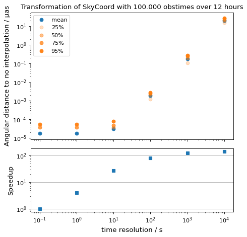
在这里,我们考虑选择合适的 time_resolution . 我们将从 ICRS 到 AltAz 并为不同的值计算精度和运行时 time_resolution 与非插值、默认方法相比。
from time import perf_counter

import numpy as np
import matplotlib.pyplot as plt

from astropy.coordinates.erfa_astrom import erfa_astrom, ErfaAstromInterpolator
from astropy.coordinates import SkyCoord, EarthLocation, AltAz
from astropy.time import Time
import astropy.units as u

rng = np.random.default_rng(1337)

# 100_000 times randomly distributed over 12 hours
t = Time('2020-01-01T20:00:00') + rng.uniform(0, 1, 10_000) * u.hour

location = EarthLocation(
    lon=-17.89 * u.deg, lat=28.76 * u.deg, height=2200 * u.m
)

# A celestial object in ICRS
crab = SkyCoord.from_name("Crab Nebula")

# target horizontal coordinate frame
altaz = AltAz(obstime=t, location=location)


# the reference transform using no interpolation
t0 = perf_counter()
no_interp = crab.transform_to(altaz)
reference = perf_counter() - t0
print(f'No Interpolation took {reference:.4f} s')


# now the interpolating approach for different time resolutions
resolutions = 10.0**np.arange(-1, 5) * u.s
times = []
seps = []

for resolution in resolutions:
    with erfa_astrom.set(ErfaAstromInterpolator(resolution)):
        t0 = perf_counter()
        interp = crab.transform_to(altaz)
        duration = perf_counter() - t0

    print(
        f'Interpolation with {resolution.value: 9.1f} {str(resolution.unit)}'
        f' resolution took {duration:.4f} s'
        f' ({reference / duration:5.1f}x faster) '
    )
    seps.append(no_interp.separation(interp))
    times.append(duration)

seps = u.Quantity(seps)

fig, (ax1, ax2) = plt.subplots(
  nrows=2,
  sharex=True,
  gridspec_kw=dict(height_ratios=[2, 1]),
)

ax1.plot(
    resolutions.to_value(u.s),
    seps.mean(axis=1).to_value(u.microarcsecond),
    'o', label='mean',
)

for p in [25, 50, 75, 95]:
    ax1.plot(
        resolutions.to_value(u.s),
        np.percentile(seps.to_value(u.microarcsecond), p, axis=1),
        'o', label=f'{p}%', color='C1', alpha=p / 100,
    )

ax1.set_title('Transformation of SkyCoord with 100.000 obstimes over 12 hours')

ax1.legend()
ax1.set_xscale('log')
ax1.set_yscale('log')
ax1.set_ylabel('Angular distance to no interpolation / µas')

ax2.plot(resolutions.to_value(u.s), reference / np.array(times), 's')
ax2.set_yscale('log')
ax2.set_ylabel('Speedup')
ax2.set_xlabel('time resolution / s')

ax2.yaxis.grid()
fig.tight_layout()

也见#
一些对理解此处所实现的坐标系的细微差别特别有用的参考包括:
- USNO Circular 179
国际天文学联盟2000/2003年围绕ICRS/IERS/CIRS开展的工作以及精密坐标系工作中的相关问题。
- Standards Of Fundamental Astronomy
IAU定义算法的最终实现。“地球态度沙发工具”文件对于详细了解国际天文学联盟最新标准特别有价值。
- IERS Conventions (2010)
一份详尽的参考文献,涵盖了ITRS,IAU2000天体坐标框架,以及现代坐标公约的其他相关细节。
- Meeus,J.“天文算法”
一个有价值的文本描述了一系列与坐标相关的问题和概念的细节。
Revisiting Spacetrack Report #3_讨论了卫星轨道的简化一般摄动(SGP),并描述了真赤道平均分点(TEME)坐标系。
内置框架和转换#
下图显示了所有内置坐标系、它们的别名(对于使用属性样式访问将其他坐标转换为它们很有用)以及它们之间的预定义转换。用户可以通过在这些系统之间定义新的转换来覆盖这些转换中的任何一个,但是预定义的转换对于典型的使用来说应该足够了。
图中边的颜色(即两帧之间的变换)由变换类型设置;图例框定义从变换类名称到颜色的映射。
-
AffineTransform: ➝
-
FunctionTransform: ➝
-
FunctionTransformWithFiniteDifference: ➝
-
StaticMatrixTransform: ➝
-
DynamicMatrixTransform: ➝
内置框架类#
ICRS系统中的坐标或框架。 |
|
FK5系统中的坐标或框架。 |
|
FK4系统中的坐标或框架。 |
|
FK4系统中的一个坐标或帧,但去掉了像差的E项。 |
|
银河系中的坐标系或坐标系。 |
|
坐标系银河系中的坐标或坐标系。 |
|
超星系坐标(见Lahav等人。 |
|
高度-方位角系统中相对于WGS84椭球体的坐标或框架(水平坐标)。 |
|
时角赤纬系统中相对于WGS84椭球体的坐标或框架(赤道坐标)。 |
|
地心天体参考系(GCRS)中的坐标或坐标系。 |
|
天球中间参考系(CIRS)中的坐标或坐标系。 |
|
国际地球参考系(ITRS)中的坐标或坐标系。 |
|
日心坐标系日心坐标系中的坐标或坐标系,轴线与ICRS对准。 |
|
真赤道平均分界线(TEME)中的坐标或坐标系。 |
|
赤道坐标使用真赤道和真春分点(TETE)的赤道坐标或坐标系。 |
|
一种坐标系,其定义与GCRS相似,但进动到要求的(平均)春分点。 |
|
地心平均黄道坐标。 |
|
重心平均黄道坐标。 |
|
日心平均黄道坐标。 |
|
地心真黄道坐标。 |
|
重心真黄道坐标。 |
|
日心真黄道坐标。 |
|
日心平均值(IAU 1976)黄道坐标。 |
|
具有自定义倾角的重心黄道坐标。 |
|
局部静止标准(LSR)中的坐标或坐标系。 |
|
运动学局部静止标准(LSR)中的坐标或坐标系。 |
|
REST的动态局部标准(LSRD)中的坐标或框架。 |
|
地方性静止标准(LSR)中的坐标或框架,与银河系框架轴对齐。 |