
时间序列 (astropy.timeseries )#
介绍#
从在固定时间对连续变量进行采样,到将事件合并到时间窗口中,天体物理学的许多不同领域都需要处理一维时间序列数据。为了满足这一需求 astropy.timeseries 子包提供表示和操作时间序列的类。
下面介绍的时间序列类是 QTable 具有特殊列的子类使用 Time 班级。因此,中描述的大部分功能 数据表 (astropy.table ) 适用于此。但是新类的主要目的是提供时间序列特定的功能 QTable .
入门#
在本节中,我们将快速了解如何读取时间序列、访问数据并执行一些基本分析。有关创建和使用时间序列的更多详细信息,请参阅中的完整文档 使用 timeseries .
最基本的时间序列类是 TimeSeries -它将时间序列表示为特定时间点的值集合。如果您对将时间序列表示为离散时间容器中的度量值感兴趣,您可能会对 BinnedTimeSeries 我们在中显示的子类 使用 timeseries )
首先,我们检索一个包含源的开普勒光曲线的FITS文件:
>>> from astropy.utils.data import get_pkg_data_filename
>>> filename = get_pkg_data_filename('timeseries/kplr010666592-2009131110544_slc.fits')
备注
此处提供的灯光曲线是出于示例目的而手工挑选的。有关开普勒配合格式的详细信息,请参见 Section 2.3.1 of the Kepler Archive Manual 。要使用Python获取其他用于科学目的的光照曲线,请参阅 astroquery 附属套餐。
然后我们可以使用 TimeSeries 要在该文件中读取的类::
>>> from astropy.timeseries import TimeSeries
>>> ts = TimeSeries.read(filename, format='kepler.fits')
时间序列是一种特殊的类型 Table 物体::
>>> ts
<TimeSeries length=14280>
          time             timecorr   ...   pos_corr1      pos_corr2
                              d       ...      pix            pix
          Time             float32    ...    float32        float32
----------------------- ------------- ... -------------- --------------
2009-05-02T00:41:40.338  6.630610e-04 ...  1.5822421e-03 -1.4463664e-03
2009-05-02T00:42:39.188  6.630857e-04 ...  1.5743829e-03 -1.4540013e-03
2009-05-02T00:43:38.045  6.631103e-04 ...  1.5665225e-03 -1.4616371e-03
2009-05-02T00:44:36.894  6.631350e-04 ...  1.5586632e-03 -1.4692718e-03
2009-05-02T00:45:35.752  6.631597e-04 ...  1.5508028e-03 -1.4769078e-03
2009-05-02T00:46:34.601  6.631844e-04 ...  1.5429436e-03 -1.4845425e-03
2009-05-02T00:47:33.451  6.632091e-04 ...  1.5350844e-03 -1.4921773e-03
2009-05-02T00:48:32.291  6.632337e-04 ...  1.5272264e-03 -1.4998110e-03
2009-05-02T00:49:31.149  6.632584e-04 ...  1.5193661e-03 -1.5074468e-03
                    ...           ... ...            ...            ...
2009-05-11T17:59:21.376  1.014518e-03 ...  3.6102540e-03  3.1872767e-03
2009-05-11T18:00:20.225  1.014542e-03 ...  3.6083264e-03  3.1795206e-03
2009-05-11T18:01:19.065  1.014567e-03 ...  3.6063993e-03  3.1717657e-03
2009-05-11T18:02:17.923  1.014591e-03 ...  3.6044715e-03  3.1640085e-03
2009-05-11T18:03:16.772  1.014615e-03 ...  3.6025438e-03  3.1562524e-03
2009-05-11T18:04:15.630  1.014640e-03 ...  3.6006160e-03  3.1484952e-03
2009-05-11T18:05:14.479  1.014664e-03 ...  3.5986886e-03  3.1407392e-03
2009-05-11T18:06:13.328  1.014689e-03 ...  3.5967610e-03  3.1329831e-03
2009-05-11T18:07:12.186  1.014713e-03 ...  3.5948332e-03  3.1252259e-03
以同样的方式 Table 对象的各个列和行 TimeSeries 可以使用索引符号访问和切片对象:
>>> ts['sap_flux']
<Quantity [1027045.06, 1027184.44, 1027076.25, ..., 1025451.56, 1025468.5 ,
           1025930.9 ] electron / s>

>>> ts['time', 'sap_flux']
<TimeSeries length=14280>
          time             sap_flux
                         electron / s
          Time             float32
----------------------- --------------
2009-05-02T00:41:40.338  1.0270451e+06
2009-05-02T00:42:39.188  1.0271844e+06
2009-05-02T00:43:38.045  1.0270762e+06
2009-05-02T00:44:36.894  1.0271414e+06
2009-05-02T00:45:35.752  1.0271569e+06
2009-05-02T00:46:34.601  1.0272296e+06
2009-05-02T00:47:33.451  1.0273199e+06
2009-05-02T00:48:32.291  1.0271497e+06
2009-05-02T00:49:31.149  1.0271755e+06
                    ...            ...
2009-05-11T17:59:21.376  1.0234574e+06
2009-05-11T18:00:20.225  1.0238128e+06
2009-05-11T18:01:19.065  1.0243234e+06
2009-05-11T18:02:17.923  1.0244257e+06
2009-05-11T18:03:16.772  1.0248654e+06
2009-05-11T18:04:15.630  1.0250156e+06
2009-05-11T18:05:14.479  1.0254516e+06
2009-05-11T18:06:13.328  1.0254685e+06
2009-05-11T18:07:12.186  1.0259309e+06

>>> ts[0:4]
<TimeSeries length=4>
          time             timecorr   ...   pos_corr1      pos_corr2
                              d       ...      pix            pix
          Time             float32    ...    float32        float32
----------------------- ------------- ... -------------- --------------
2009-05-02T00:41:40.338  6.630610e-04 ...  1.5822421e-03 -1.4463664e-03
2009-05-02T00:42:39.188  6.630857e-04 ...  1.5743829e-03 -1.4540013e-03
2009-05-02T00:43:38.045  6.631103e-04 ...  1.5665225e-03 -1.4616371e-03
2009-05-02T00:44:36.894  6.631350e-04 ...  1.5586632e-03 -1.4692718e-03
如前面的例子所示, TimeSeries 对象有一个 time 列,它始终是第一列。也可以使用 .time 属性:
>>> ts.time
<Time object: scale='tdb' format='isot' value=['2009-05-02T00:41:40.338' '2009-05-02T00:42:39.188'
  '2009-05-02T00:43:38.045' ... '2009-05-11T18:05:14.479'
  '2009-05-11T18:06:13.328' '2009-05-11T18:07:12.186']>
第一列总是 Time 对象(参见 Times and Dates ),因此支持转换为不同时间尺度和格式的能力:
>>> ts.time.mjd
array([54953.0289391 , 54953.02962023, 54953.03030145, ...,
       54962.7536398 , 54962.75432093, 54962.75500215])

>>> ts.time.unix
array([1.24122483e+09, 1.24122489e+09, 1.24122495e+09, ...,
       1.24206505e+09, 1.24206511e+09, 1.24206517e+09])
我们还可以检查时间定义的时间刻度:
>>> ts.time.scale
'tdb'
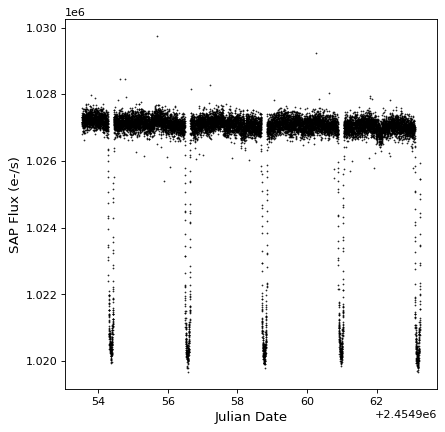
这是重心动力学时间尺度(参见 时间和日期 (astropy.time ) 更多细节)。我们可以用我们目前所看到的来制作一个情节:
import matplotlib.pyplot as plt
plt.plot(ts.time.jd, ts['sap_flux'], 'k.', markersize=1)
plt.xlabel('Julian Date')
plt.ylabel('SAP Flux (e-/s)')

看起来好像有几个过境点!我们可以使用 BoxLeastSquares 类来使用“盒最小二乘法”(BLS)算法估计周期:
>>> import numpy as np
>>> from astropy import units as u
>>> from astropy.timeseries import BoxLeastSquares
>>> periodogram = BoxLeastSquares.from_timeseries(ts, 'sap_flux')
要运行周期图分析,我们使用一个持续时间为0.2天的框:
>>> results = periodogram.autopower(0.2 * u.day)
>>> best = np.argmax(results.power)
>>> period = results.period[best]
>>> period
<Quantity 2.20551724 d>
>>> transit_time = results.transit_time[best]
>>> transit_time
<Time object: scale='tdb' format='isot' value=2009-05-02T20:51:16.338>
有关可用周期图算法的详细信息,请参阅 周期图算法 .
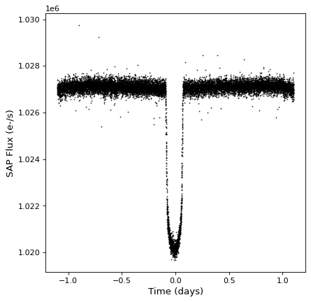
我们现在可以使用上面找到的时间段来折叠时间序列 fold() 方法:
>>> ts_folded = ts.fold(period=period, epoch_time=transit_time)
现在我们可以看看折叠的时间序列:
plt.plot(ts_folded.time.jd, ts_folded['sap_flux'], 'k.', markersize=1)
plt.xlabel('Time (days)')
plt.ylabel('SAP Flux (e-/s)')

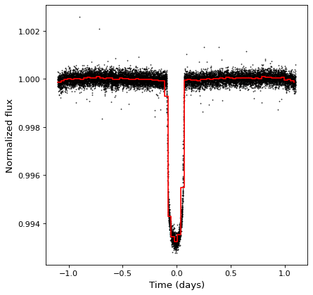
使用 天体统计工具 (astropy.stats ) 模块,我们可以通过sigma剪裁数据来规范化通量,以确定基线通量:
>>> from astropy.stats import sigma_clipped_stats
>>> mean, median, stddev = sigma_clipped_stats(ts_folded['sap_flux'])
>>> ts_folded['sap_flux_norm'] = ts_folded['sap_flux'] / median
我们可以通过将这些点划分为相等时间的单元来降低时间序列的采样率-这将返回一个 BinnedTimeSeries ::
>>> from astropy.timeseries import aggregate_downsample
>>> ts_binned = aggregate_downsample(ts_folded, time_bin_size=0.03 * u.day)
>>> ts_binned
<BinnedTimeSeries length=74>
   time_bin_start   time_bin_size ...       pos_corr2          sap_flux_norm
                          d       ...          pix
     TimeDelta         float64    ...        float64              float64
------------------- ------------- ... ---------------------- ------------------
-1.1022116370482966          0.03 ... 0.00031207725987769663 0.9998741745948792
-1.0722116370482966          0.03 ... 0.00041217938996851444 0.9999074339866638
-1.0422116370482966          0.03 ... 0.00039273229776881635  0.999972939491272
-1.0122116370482965          0.03 ...  0.0002928022004198283 1.0000077486038208
-0.9822116370482965          0.03 ...  0.0003891147789545357 0.9999921917915344
-0.9522116370482965          0.03 ...  0.0003491091774776578 1.0000101327896118
-0.9222116370482966          0.03 ...  0.0002824827388394624 1.0000121593475342
-0.8922116370482965          0.03 ... 0.00016335179680027068 0.9999905228614807
-0.8622116370482965          0.03 ...  0.0001397567830281332 1.0000263452529907
                ...           ... ...                    ...                ...
  0.847788362951705          0.03 ... 0.00022221534163691103 1.0000633001327515
  0.877788362951705          0.03 ... 0.00019213277846574783 1.0000433921813965
 0.9077883629517051          0.03 ...  0.0002187517675338313  1.000024676322937
 0.9377883629517049          0.03 ... 0.00016979355132207274 1.0000224113464355
 0.9677883629517047          0.03 ... 0.00014231358363758773 1.0000698566436768
 0.9977883629517045          0.03 ...  0.0001224415173055604 0.9999606013298035
 1.0277883629517042          0.03 ... 0.00027701034559868276 0.9999635815620422
  1.057788362951704          0.03 ...  0.0003093520936090499 0.9999105930328369
 1.0877883629517038          0.03 ... 0.00022884277859702706 0.9998687505722046
现在我们可以看看最终结果:
plt.plot(ts_folded.time.jd, ts_folded['sap_flux_norm'], 'k.', markersize=1)
plt.plot(ts_binned.time_bin_start.jd, ts_binned['sap_flux_norm'], 'r-', drawstyle='steps-post')
plt.xlabel('Time (days)')
plt.ylabel('Normalized flux')

进一步了解 astropy.timeseries 模块,您可以在下一节中找到指向完整文档的链接。
使用 timeseries#
使用细节 astropy.timeseries 在以下章节中提供: