
时间序列的处理与分析#
组合时间序列#
这个 vstack() 和 hstack() 中的函数 astropy.table 模块可用于以不同方式堆叠时间序列。
实例#
使用 vstack() 函数(注意采样时间序列不能与二进制时间序列组合,反之亦然):
>>> from astropy.table import vstack
>>> from astropy import units as u
>>> from astropy.timeseries import TimeSeries
>>> ts_a = TimeSeries(time_start='2016-03-22T12:30:31',
...                   time_delta=3 * u.s,
...                   data={'flux': [1, 4, 5, 3, 2] * u.mJy})
>>> ts_b = TimeSeries(time_start='2016-03-22T12:50:31',
...                   time_delta=3 * u.s,
...                   data={'flux': [4, 3, 1, 2, 3] * u.mJy})
>>> ts_ab = vstack([ts_a, ts_b])
>>> ts_ab
<TimeSeries length=10>
          time            flux
                          mJy
          Time          float64
----------------------- -------
2016-03-22T12:30:31.000     1.0
2016-03-22T12:30:34.000     4.0
2016-03-22T12:30:37.000     5.0
2016-03-22T12:30:40.000     3.0
2016-03-22T12:30:43.000     2.0
2016-03-22T12:50:31.000     4.0
2016-03-22T12:50:34.000     3.0
2016-03-22T12:50:37.000     1.0
2016-03-22T12:50:40.000     2.0
2016-03-22T12:50:43.000     3.0
注意 vstack() 不会自动排序,也不会清除重复项—这是您以后需要显式执行的操作。
也可以使用 hstack() 函数,但这些不应该是时间序列(因为有多个时间列会令人困惑):
>>> from astropy.table import Table, hstack
>>> data = Table(data={'temperature': [40., 41., 40., 39., 30.] * u.K})
>>> ts_a_data = hstack([ts_a, data])
>>> ts_a_data
<TimeSeries length=5>
          time            flux  temperature
                          mJy          K
          Time          float64    float64
----------------------- ------- -----------
2016-03-22T12:30:31.000     1.0        40.0
2016-03-22T12:30:34.000     4.0        41.0
2016-03-22T12:30:37.000     5.0        40.0
2016-03-22T12:30:40.000     3.0        39.0
2016-03-22T12:30:43.000     2.0        30.0
排序时间序列#
>>> ts = TimeSeries(time_start='2016-03-22T12:30:31',
...                 time_delta=3 * u.s,
...                 data={'flux': [1., 4., 5., 3., 2.]})
>>> ts
<TimeSeries length=5>
          time            flux
          Time          float64
----------------------- -------
2016-03-22T12:30:31.000     1.0
2016-03-22T12:30:34.000     4.0
2016-03-22T12:30:37.000     5.0
2016-03-22T12:30:40.000     3.0
2016-03-22T12:30:43.000     2.0
>>> ts.sort('flux')
>>> ts
<TimeSeries length=5>
          time            flux
          Time          float64
----------------------- -------
2016-03-22T12:30:31.000     1.0
2016-03-22T12:30:43.000     2.0
2016-03-22T12:30:40.000     3.0
2016-03-22T12:30:34.000     4.0
2016-03-22T12:30:37.000     5.0
重采样#
我们为您提供一个 aggregate_downsample() 一种函数,可用于使用自定义函数(平均值、中位数等)将时间序列中的值分成大小相等或不均匀的分块,以及连续和非连续分块。此操作返回一个 BinnedTimeSeries 。请注意,这是一个基本函数,例如,它不知道如何将具有不确定性的列与其他值区别对待,并且它将盲目地将指定的定制函数应用于所有列。
例子#
下面的示例显示如何使用 aggregate_downsample() 使用中值函数将开普勒任务中的光曲线分成20分钟连续的分块。首先,我们使用以下方法读入数据:
from astropy.timeseries import TimeSeries
from astropy.utils.data import get_pkg_data_filename
example_data = get_pkg_data_filename('timeseries/kplr010666592-2009131110544_slc.fits')
kepler = TimeSeries.read(example_data, format='kepler.fits', unit_parse_strict='silent')
(见 读写时间序列 有关读取数据的更多详细信息)。然后,我们可以使用以下方法减少采样:
import numpy as np
from astropy import units as u
from astropy.timeseries import aggregate_downsample
kepler_binned = aggregate_downsample(kepler, time_bin_size=20 * u.min, aggregate_func=np.nanmedian)
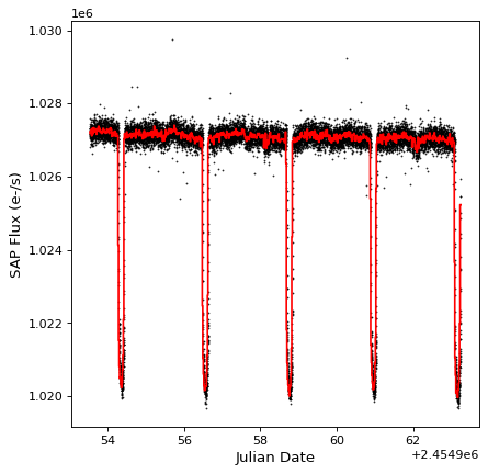
我们可以看看结果:
import matplotlib.pyplot as plt
fig, ax = plt.subplots()
ax.plot(kepler.time.jd, kepler['sap_flux'], 'k.', markersize=1)
ax.plot(kepler_binned.time_bin_start.jd, kepler_binned['sap_flux'], 'r-', drawstyle='steps-pre')
ax.set(xlabel='Julian Date', ylabel='SAP Flux (e-/s)')
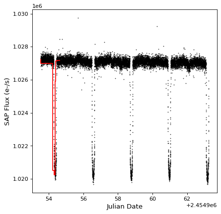
这个 aggregate_downsample() 也可用于将灯光曲线绑定到自定义存储箱中。下面的示例显示大小不均匀的连续垃圾桶的情况:
kepler_binned = aggregate_downsample(kepler, time_bin_size=[1000, 125, 80, 25, 150, 210, 273] * u.min,
                                     aggregate_func=np.nanmedian)

fig, ax = plt.subplots()
ax.plot(kepler.time.jd, kepler['sap_flux'], 'k.', markersize=1)
ax.plot(kepler_binned.time_bin_start.jd, kepler_binned['sap_flux'], 'r-', drawstyle='steps-pre')
ax.set(xlabel='Julian Date', ylabel='SAP Flux (e-/s)')

要了解有关自定义绑定功能的详细信息,请参阅 aggregate_downsample() ,见 初始化二进制时间序列 。
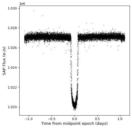
折叠#
这个 TimeSeries 类有 fold() 方法,该方法可用于返回具有相对和折叠时间轴的新时间序列。此方法将周期作为 Quantity ,并且可以选择将一个纪元作为 Time ,它定义了零时间偏移:
kepler_folded = kepler.fold(period=2.2 * u.day, epoch_time='2009-05-02T20:53:40')

fig, ax = plt.subplots()
ax.plot(kepler_folded.time.jd, kepler_folded['sap_flux'], 'k.', markersize=1)
ax.set(xlabel='Time from midpoint epoch (days)', ylabel='SAP Flux (e-/s)')

注意,在这个例子中,我们碰巧从之前的周期图分析中知道了周期和中点。请参见中的示例 时间序列 (astropy.timeseries ) 你会怎么做的。
算术#
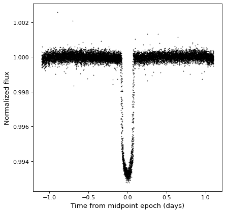
自从 TimeSeries 对象是的子类 Table ,它们自然支持任何数据列上的算术运算。作为一个例子,我们可以取前面例子中看到的折叠开普勒时间序列,并将其规范化为sigma剪裁中值。
from astropy.stats import sigma_clipped_stats

mean, median, stddev = sigma_clipped_stats(kepler_folded['sap_flux'])

kepler_folded['sap_flux_norm'] = kepler_folded['sap_flux'] / median

fig, ax = plt.subplots()
ax.plot(kepler_folded.time.jd, kepler_folded['sap_flux_norm'], 'k.', markersize=1)
ax.set(xlabel='Time from midpoint epoch (days)', ylabel='Normalized flux')