组合模型

基础

而Astropy建模包使其非常容易定义 new models 从现有函数，或通过编写 Model 子类，创建新模型的另一种方法是使用算术表达式组合它们。这适用于Astropy中内置的模型，以及大多数用户定义的模型。例如，可以创建两个高斯的叠加，如下所示：

>>> from astropy.modeling import models
>>> g1 = models.Gaussian1D(1, 0, 0.2)
>>> g2 = models.Gaussian1D(2.5, 0.5, 0.1)
>>> g1_plus_2 = g1 + g2

生成的对象 g1_plus_2 本身就是一种新的模式。

备注

模型 g1_plus_2 is a CompoundModel which contains the models g1 and g2 without any parameter duplication. Meaning changes to the parameters of g1_plus_2 will effect the parameters of g1 or g2 and vice versa; if one does not want this to occur one can copy the models prior to adding them using the .copy() method g1.copy() + g2.copy(). In general applies to any CompoundModel constructed using a binary operation, so that CompoundModel follows the Python convention for construction of container objects. For more information on this please see the API Changes in astropy.modeling

评估，比如说， g1_plus_2(0.25) 等同于评估 g1(0.25) + g2(0.25) **

>>> g1_plus_2(0.25)  
0.5676756958301329
>>> g1_plus_2(0.25) == g1(0.25) + g2(0.25)
True

该模型可以与其他模型进一步组合成新的表达式。

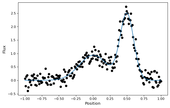
与大多数其他模型一样，这些新的复合模型也可以拟合数据（尽管目前这需要一个非线性拟合器）：

import warnings
import numpy as np
import matplotlib.pyplot as plt
from astropy.modeling import models, fitting

# Generate fake data
rng = np.random.default_rng(seed=42)
g1 = models.Gaussian1D(1, 0, 0.2)
g2 = models.Gaussian1D(2.5, 0.5, 0.1)
x = np.linspace(-1, 1, 200)
y = g1(x) + g2(x) + rng.normal(0., 0.2, x.shape)

# Now to fit the data create a new superposition with initial
# guesses for the parameters:
gg_init = models.Gaussian1D(1, 0, 0.1) + models.Gaussian1D(2, 0.5, 0.1)
fitter = fitting.SLSQPLSQFitter()

with warnings.catch_warnings():
    # Ignore a warning on clipping to bounds from the fitter
    warnings.filterwarnings('ignore', message='Values in x were outside bounds',
                            category=RuntimeWarning)
    gg_fit = fitter(gg_init, x, y)

# Plot the data with the best-fit model
plt.figure(figsize=(8,5))
plt.plot(x, y, 'ko')
plt.plot(x, gg_fit(x))
plt.xlabel('Position')
plt.ylabel('Flux')

(png, svg, pdf)

这种方法适用于1-D模型、2-D模型及其组合，尽管正确匹配用于构建复合模型的所有模型的输入和输出有一些复杂性。您可以在 组合模型 文档。

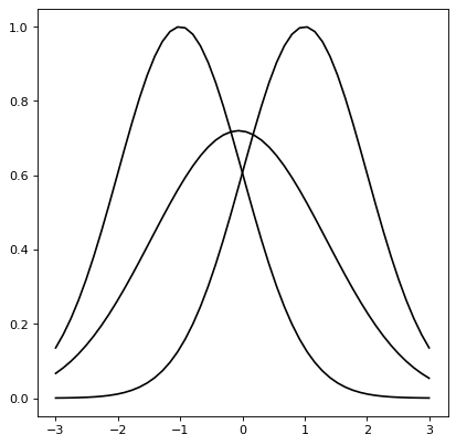
Astropy模型还支持通过函数进行卷积 convolve_models ，返回一个复合模型。

例如，两个高斯函数的卷积也是一个高斯函数，其中得到的平均值（方差）是每个高斯函数的平均值（方差）之和。

import numpy as np
import matplotlib.pyplot as plt
from astropy.modeling import models
from astropy.convolution import convolve_models

g1 = models.Gaussian1D(1, -1, 1)
g2 = models.Gaussian1D(1, 1, 1)
g3 = convolve_models(g1, g2)

x = np.linspace(-3, 3, 50)
plt.plot(x, g1(x), 'k-')
plt.plot(x, g2(x), 'k-')
plt.plot(x, g3(x), 'k-')

(png, svg, pdf)

全面的描述

一些术语

只需使用算术运算符组合现有模型，就可以创建新的模型 +, -, *, /, and `` **，或使用 ``| 和连接（如下所述）与 & ，以及使用 fix_inputs() 对于 reducing the number of inputs to a model .

在讨论复合模型特性时，有必要明确一些存在混淆点的术语：

• 术语“模型”可以指模型 类 或者一个模型 实例 .

  • 所有型号 astropy.modeling ，无论它是否代表 function ，A rotation 等等，在抽象中用一个模型表示 类 --特别是 Model --它封装了评估模型的例程、所需参数的列表以及有关模型的其他元数据。

  • 按照典型的面向对象的说法，一个模型 实例 是在调用带有某些参数的模型类时创建的对象，在大多数情况下是模型参数的值。

  模型类本身不能用于执行任何计算，因为大多数模型至少都有一个或多个参数，这些参数必须在对某些输入数据进行计算之前指定。但是，我们仍然可以从模型类的表示中获得一些有关它的信息。例如：：

  >>> from astropy.modeling.models import Gaussian1D
  >>> Gaussian1D
  <class 'astropy.modeling.functional_models.Gaussian1D'>
  Name: Gaussian1D
  N_inputs: 1
  N_outputs: 1
  Fittable parameters: ('amplitude', 'mean', 'stddev')
  

  然后我们可以创建一个模型 实例 通过传入三个参数的值：

  >>> my_gaussian = Gaussian1D(amplitude=1.0, mean=0, stddev=0.2)
  >>> my_gaussian  
  <Gaussian1D(amplitude=1.0, mean=0.0, stddev=0.2)>
  

  我们现在有一个 实例 属于 Gaussian1D 它的所有参数（原则上还有其他细节，如拟合约束）都已填写，以便我们可以像函数一样使用它进行计算：

  >>> my_gaussian(0.2)  
  0.6065306597126334
  

  在许多情况下，本文档只提到“模型”，其中类/实例的区别要么无关紧要，要么与上下文无关。但在必要的时候会做出区分。

• A compound model 可以通过组合两个或更多现有模型实例来创建，这些模型实例可以是Astropy附带的模型， user defined models 或其他复合模型--使用由一个或多个受支持的二元运算符组成的Python表达式。

• 在某些地方 复合模型 可与互换使用 复合模型 . 然而，本文件使用了术语 复合模型 参考 only 对于使用管道操作符从两个或多个模型的功能组合创建的复合模型的情况 | 如下所述。此区别在本文档中一直使用，但理解其区别可能会有所帮助。

创建复合模型

创建复合模型的唯一方法是使用Python中的表达式和二进制运算符组合现有的单个模型和/或复合模型 +, -, *, /, `` **, ``| 和 & ，以下各节将对此进行讨论。

组合两个模型的结果是一个模型实例：

>>> two_gaussians = Gaussian1D(1.1, 0.1, 0.2) + Gaussian1D(2.5, 0.5, 0.1)
>>> two_gaussians  
<CompoundModel...(amplitude_0=1.1, mean_0=0.1, stddev_0=0.2, amplitude_1=2.5, mean_1=0.5, stddev_1=0.1)>

此表达式创建一个新的模型实例，该实例可用于计算：

>>> two_gaussians(0.2)  
0.9985190841886609

这个 print 函数提供有关此对象的详细信息：

>>> print(two_gaussians)
Model: CompoundModel...
Inputs: ('x',)
Outputs: ('y',)
Model set size: 1
Expression: [0] + [1]
Components:
    [0]: <Gaussian1D(amplitude=1.1, mean=0.1, stddev=0.2)>

    [1]: <Gaussian1D(amplitude=2.5, mean=0.5, stddev=0.1)>
Parameters:
    amplitude_0 mean_0 stddev_0 amplitude_1 mean_1 stddev_1
    ----------- ------ -------- ----------- ------ --------
            1.1    0.1      0.2         2.5    0.5      0.1

这里有很多事情需要指出：这个模型有六个合适的参数。参数的处理方式将在 参数 . 我们还可以看到 表达 用于创建此复合模型的 [0] + [1] . 这个 [0] 和 [1] 参考下面列出的模型的第一个和第二个组件（在这种情况下，两个组件都是 Gaussian1D 对象）。

复合模型的每个组件都是一个单独的非复合模型。即使在新表达式中包含现有的复合模型也是如此。现有的复合模型不被视为单个模型，而是扩展了由该复合模型表示的表达式。包含两个或多个复合模型的表达式将生成一个新表达式，该表达式是所有相关模型表达式的串联：

>>> four_gaussians = two_gaussians + two_gaussians
>>> print(four_gaussians)
Model: CompoundModel...
Inputs: ('x',)
Outputs: ('y',)
Model set size: 1
Expression: [0] + [1] + [2] + [3]
Components:
    [0]: <Gaussian1D(amplitude=1.1, mean=0.1, stddev=0.2)>

    [1]: <Gaussian1D(amplitude=2.5, mean=0.5, stddev=0.1)>

    [2]: <Gaussian1D(amplitude=1.1, mean=0.1, stddev=0.2)>

    [3]: <Gaussian1D(amplitude=2.5, mean=0.5, stddev=0.1)>
Parameters:
    amplitude_0 mean_0 stddev_0 amplitude_1 ... stddev_2 amplitude_3 mean_3 stddev_3
    ----------- ------ -------- ----------- ... -------- ----------- ------ --------
            1.1    0.1      0.2         2.5 ...      0.2         2.5    0.5      0.1

算子

算术运算符

复合模型可以从包含任意数量算术运算符的表达式中创建 +, -, *, /, and `` **``在Python中，它们与其他对象具有相同的数字含义。

备注

在分割的情况下 / 总是指浮点除法——整数除法和 // 模型不支持运算符）。

如前面的示例所示，对于具有单个输出的模型，评估模型的结果如下所示 A + B 是为了评估 A 和 B 分别对给定的输入，然后返回 A 和 B . 这就要求 A 和 B 采用相同数量的输入，两个都有一个输出。

也可以在具有多个输出的模型之间使用算术运算符。同样，模型之间的输入数量必须相同，输出数量也必须相同。在本例中，运算符按元素应用于运算符，类似于算术运算符在两个Numpy数组上的工作方式。

模型组成

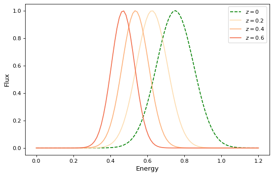
可用于创建复合模型的第六个二进制运算符是复合运算符，也称为“管道”运算符 | （不要与它为Python数字对象实现的boolean“or”运算符混淆）。使用组合运算符创建的模型，如 M = F | G ，在计算时，相当于计算 \(g \circ f = g(f(x))\) .

备注

事实上， | 运算符与函数复合运算符的含义相反 \(\circ\) 有时是一个混乱点。这在一定程度上是因为Python中不支持与此对应的运算符符号。这个 | 运算符应改为 pipe operator unixshell语法：它通过管道将左侧操作数的输出与右侧操作数的输入连接起来，形成模型或转换的“管道”。

与算术运算符相比，它对操作数的输入/输出有不同的要求。对于合成，所需要的只是左侧模型具有与右侧模型具有相同数量的输入的输出。

对于简单的函数模型，这与函数组合完全相同，除了前面提到的关于排序的警告。例如，要创建以下复合模型：

import numpy as np
import matplotlib.pyplot as plt
from astropy.modeling.models import RedshiftScaleFactor, Gaussian1D

x = np.linspace(0, 1.2, 100)
g0 = RedshiftScaleFactor(0) | Gaussian1D(1, 0.75, 0.1)

plt.figure(figsize=(8, 5))
plt.plot(x, g0(x), 'g--', label='$z=0$')

for z in (0.2, 0.4, 0.6):
    g = RedshiftScaleFactor(z) | Gaussian1D(1, 0.75, 0.1)
    plt.plot(x, g(x), color=plt.cm.OrRd(z),
             label=f'$z={z}$')

plt.xlabel('Energy')
plt.ylabel('Flux')
plt.legend()

(png, svg, pdf)

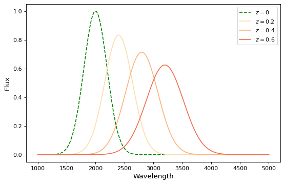
如果您希望在波长空间而不是能量上执行红移，并且还希望保存通量，这里有另一种使用模型的方法 实例 ：

import numpy as np
import matplotlib.pyplot as plt
from astropy.modeling.models import RedshiftScaleFactor, Gaussian1D, Scale

x = np.linspace(1000, 5000, 1000)
g0 = Gaussian1D(1, 2000, 200)  # No redshift is same as redshift with z=0

plt.figure(figsize=(8, 5))
plt.plot(x, g0(x), 'g--', label='$z=0$')

for z in (0.2, 0.4, 0.6):
    rs = RedshiftScaleFactor(z).inverse  # Redshift in wavelength space
    sc = Scale(1. / (1 + z))  # Rescale the flux to conserve energy
    g = rs | g0 | sc
    plt.plot(x, g(x), color=plt.cm.OrRd(z),
             label=f'$z={z}$')

plt.xlabel('Wavelength')
plt.ylabel('Flux')
plt.legend()

(png, svg, pdf)

当使用具有多个输入和输出的模型时，同样的想法也适用。如果每个输入都被认为是一个坐标轴，那么这就为每个轴上的坐标定义了一个转换管道（尽管它不一定保证这些转换是可分离的）。例如：

import numpy as np
import matplotlib.pyplot as plt
from astropy.modeling.models import Rotation2D, Gaussian2D

x, y = np.mgrid[-1:1:0.01, -1:1:0.01]

plt.figure(figsize=(8, 2.5))

for idx, theta in enumerate((0, 45, 90)):
    g = Rotation2D(theta) | Gaussian2D(1, 0, 0, 0.1, 0.3)
    plt.subplot(1, 3, idx + 1)
    plt.imshow(g(x, y), origin='lower')
    plt.xticks([])
    plt.yticks([])
    plt.title(rf'Rotated $ {theta}^\circ $')

(png, svg, pdf)

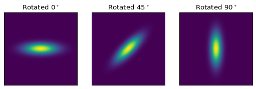
备注

上面的例子有点做作 Gaussian2D 已经支持可选的旋转参数。然而，这演示了如何将坐标旋转添加到任意模型中。

通常情况下，不可能组成一个有两个输出和只有一个输入函数的模型：

>>> from astropy.modeling.models import Rotation2D
>>> Rotation2D() | Gaussian1D()  
Traceback (most recent call last):
...
ModelDefinitionError: Unsupported operands for |: Rotation2D (n_inputs=2, n_outputs=2) and Gaussian1D (n_inputs=1, n_outputs=1); n_outputs for the left-hand model must match n_inputs for the right-hand model.

然而，正如我们将在下一节中看到的， 模型串联 提供了一种创建模型的方法，这些模型只将转换应用于模型的某些输出，特别是在与 mappings .

模型串联

串联运算符 & ，有时也称为“连接”，将两个模型组合为一个完全可分离的转换。也就是说，它创建了一个新模型，该模型接受左侧模型的输入，与右侧模型的输入连接，并返回一个元组，该元组由连接在一起的两个模型的输出组成，而不会以任何方式混合。换句话说，它只是并行地计算两个模型——它可以被看作是模型的元组。

例如，给定两个坐标轴，我们可以通过连接两个坐标轴来按不同的因子缩放每个坐标 Scale 模型。

>>> from astropy.modeling.models import Scale
>>> separate_scales = Scale(factor=1.2) & Scale(factor=3.4)
>>> separate_scales(1, 2)  
(1.2, 6.8)

我们还可以将串联与组合结合起来，构建在两个（或更多）坐标轴上同时使用“1D”和“2D”模型的转换链：

>>> scale_and_rotate = ((Scale(factor=1.2) & Scale(factor=3.4)) |
...                     Rotation2D(90))
>>> scale_and_rotate.n_inputs
2
>>> scale_and_rotate.n_outputs
2
>>> scale_and_rotate(1, 2)  
(-6.8, 1.2)

这当然相当于 AffineTransformation2D 使用适当的变换矩阵：

>>> from numpy import allclose
>>> from astropy.modeling.models import AffineTransformation2D
>>> affine = AffineTransformation2D(matrix=[[0, -3.4], [1.2, 0]])
>>> # May be small numerical differences due to different implementations
>>> allclose(scale_and_rotate(1, 2), affine(1, 2))
True

其他主题

型号名称

在上面两个例子中，生成的复合模型类的另一个显著特征是，在命令提示符下打印类时显示的类名不是“twogussians”，“FourGaussians”，相反，它是一个生成的名称，由“CompoundModel”后跟一个基本上任意的整数组成，这样每个复合模型都有一个唯一的默认名称。这是目前的一个限制，因为在Python中，当一个对象由表达式创建时，它通常不可能“知道”它将被赋给的变量的名称（如果有的话）。可以使用 Model.name 属性：

>>> two_gaussians.name = "TwoGaussians"
>>> print(two_gaussians)  
Model: CompoundModel...
Name: TwoGaussians
Inputs: ('x',)
Outputs: ('y',)
Model set size: 1
Expression: [0] + [1]
Components:
    [0]: <Gaussian1D(amplitude=1.1, mean=0.1, stddev=0.2)>

    [1]: <Gaussian1D(amplitude=2.5, mean=0.5, stddev=0.1)>
Parameters:
    amplitude_0 mean_0 stddev_0 amplitude_1 mean_1 stddev_1
    ----------- ------ -------- ----------- ------ --------
            1.1    0.1      0.2         2.5    0.5      0.1

索引和切片

如本文前面的一些示例所示，当创建复合模型时，模型的每个组件都被分配一个从零开始的整数索引。这些索引只需通过从左到右读取定义模型的表达式来赋值，而不考虑操作的顺序。例如：：

>>> from astropy.modeling.models import Const1D
>>> A = Const1D(1.1, name='A')
>>> B = Const1D(2.1, name='B')
>>> C = Const1D(3.1, name='C')
>>> M = A + B * C
>>> print(M)
Model: CompoundModel...
Inputs: ('x',)
Outputs: ('y',)
Model set size: 1
Expression: [0] + [1] * [2]
Components:
    [0]: <Const1D(amplitude=1.1, name='A')>

    [1]: <Const1D(amplitude=2.1, name='B')>

    [2]: <Const1D(amplitude=3.1, name='C')>
Parameters:
    amplitude_0 amplitude_1 amplitude_2
    ----------- ----------- -----------
            1.1         2.1         3.1

在本例中，计算表达式 (B * C) + A --也就是说，乘法运算在加法运算之前根据通常的算术规则进行计算。但是，这个模型的组件只是从表达式中从左到右读取 A + B * C 用 A -> 0 ， B -> 1 ， C -> 2 . 如果我们定义 M = C * B + A 然后，索引将被反转（尽管表达式在数学上是等价的）。选择这个约定是为了简单起见——考虑到组件的列表，在将它们映射到表达式时，不需要跳来跳去。

我们可以找出复合模型的每个单独的组成部分 M 使用索引符号。根据上面的例子， M[1] 应该返回模型 B ：：

>>> M[1]
<Const1D(amplitude=2.1, name='B')>

我们也可以 片 复合模型的。这将返回一个新的复合模型，该模型计算 子表达式 包括切片选择的模型。这与切片a的语义相同 list 或者Python中的数组。起点是包容的，终点是排他的。所以一片 M[1:3] （或者只是 M[1:] )选择模型 B 和 C （以及所有 算子 在他们之间）。因此，结果模型只计算子表达式 B * C ：：

>>> print(M[1:])
Model: CompoundModel
Inputs: ('x',)
Outputs: ('y',)
Model set size: 1
Expression: [0] * [1]
Components:
    [0]: <Const1D(amplitude=2.1, name='B')>

    [1]: <Const1D(amplitude=3.1, name='C')>
Parameters:
    amplitude_0 amplitude_1
    ----------- -----------
            2.1         3.1

备注

在4.0之前的版本中，切片的参数名发生了更改。以前，参数名称与被切片的模型的名称相同。现在，除了切片的模型之外，它们是这种类型的复合模型所期望的。也就是说，切片模型总是以其组件的相对索引开始，因此参数名以0后缀开头。

备注

从4.0开始，切片的行为比以前更加严格。例如，如果：

m = m1 * m2 + m3

还有一个是用 m[1:3] 之前会返回模型： m2 + m3 尽管m从来没有这样的子模型。从4.0开始，一个切片必须对应于一个子模型（与计算复合模型的计算链的中间结果相对应）。所以：

m1 * m2

是一个子模型（即`m [:2] )但是 ``m[1:3] 不是。目前，这也意味着在更简单的表达式中，例如：

m = m1 + m2 + m3 + m4

如果任何切片原则上都是有效的，那么只有包含m1的切片是因为它是所有子模块的一部分（因为求值顺序是：：

((m1 + m2) + m3) + m4

建议任何创建复合模型并希望子模型可用的人显式使用括号，或者定义要在后续表达式中使用的中间模型，以便可以根据上下文使用切片或简单索引提取它们。例如，使 m2 + m3 按切片定义访问 m AS：：

m = m1 + (m2 + m3) + m4. In this case ``m[1:3]`` will work.

子表达式的新复合模型可以像任何其他模型一样进行计算：

>>> M[1:](0)  
6.51

虽然模型 M 完全由 Const1D 在这个例子中，给每个组件一个唯一的名称是很有用的 (A ， B ， C )为了区分它们。这也可以用于索引和切片：

>>> print(M['B'])
Model: Const1D
Name: B
Inputs: ('x',)
Outputs: ('y',)
Model set size: 1
Parameters:
    amplitude
    ---------
          2.1

在这种情况下 M['B'] 相当于 M[1] 。但是通过使用名称，我们不必担心该组件在哪个索引中(这在组合多个复合模型时变得特别有用)。然而，当前的限制是复合模型的每个组件必须具有唯一的名称--如果某些组件具有重复的名称，则它们只能通过其整数索引进行访问。

切片也适用于名称。使用名称时，起点和终点是 两者兼而有之 ：：

>>> print(M['B':'C'])
Model: CompoundModel...
Inputs: ('x',)
Outputs: ('y',)
Model set size: 1
Expression: [0] * [1]
Components:
    [0]: <Const1D(amplitude=2.1, name='B')>

    [1]: <Const1D(amplitude=3.1, name='C')>
Parameters:
    amplitude_0 amplitude_1
    ----------- -----------
            2.1         3.1

所以在这种情况下 M['B':'C'] 等于 M[1:3] .

参数

当第一次遇到复合模型时，经常会出现一个问题，即所有参数是如何精确处理的。到目前为止，我们已经看到了一些给出了一些提示的示例，但是需要更详细的解释。这也是可能改进的最大领域之一——当前的行为是为了实用，但并不理想。（一些可能的改进包括能够重命名参数，以及提供一种缩小复合模型中参数数量的方法。）

如模型通用文档中所述 parameters ，每个模型都有一个名为 param_names 它包含模型所有可调参数的元组。这些名称以规范的顺序给出，该顺序也与实例化模型时指定参数的顺序相对应。

当前用于命名复合模型中参数的简单方案是： param_names 从每个组件模型按从左到右的顺序相互连接，如上一节中所述 索引和切片 . 但是，每个参数名都附加有 _<#> 在哪里 <#> 参数所属组件模型的索引。例如：：

>>> Gaussian1D.param_names
('amplitude', 'mean', 'stddev')
>>> (Gaussian1D() + Gaussian1D()).param_names
('amplitude_0', 'mean_0', 'stddev_0', 'amplitude_1', 'mean_1', 'stddev_1')

为了保持一致性，即使不是所有组件都有重叠的参数名，也会遵循此方案：

>>> from astropy.modeling.models import RedshiftScaleFactor
>>> (RedshiftScaleFactor() | (Gaussian1D() + Gaussian1D())).param_names
('z_0', 'amplitude_1', 'mean_1', 'stddev_1', 'amplitude_2', 'mean_2',
'stddev_2')

在某种程度上，为了使复合模型在其参数的接口上与其他模型保持一定的一致性，这样的方案是必要的。然而，如果一个人迷路了，也可以利用它 indexing 让事情更简单。从复合模型返回单个组件时，与该组件关联的参数可以通过其原始名称进行访问，但仍绑定到复合模型：

>>> a = Gaussian1D(1, 0, 0.2, name='A')
>>> b = Gaussian1D(2.5, 0.5, 0.1, name='B')
>>> m = a + b
>>> m.amplitude_0
Parameter('amplitude', value=1.0)

等于：

>>> m['A'].amplitude
Parameter('amplitude', value=1.0)

你可以把这两者看作是同一参数的不同“视图”。更新一个更新另一个：

>>> m.amplitude_0 = 42
>>> m['A'].amplitude
Parameter('amplitude', value=42.0)
>>> m['A'].amplitude = 99
>>> m.amplitude_0
Parameter('amplitude', value=99.0)

但是，请注意，原始的 Gaussian1D 实例 a 已更新：

>>> a.amplitude
Parameter('amplitude', value=99.0)

这与4.0之前版本中的行为不同。现在，复合模型参数与原始模型共享相同的参数实例。

高级映射

在前面的一些示例中，我们已经看到了如何使用模型将模型链接在一起以形成转换的“管道” composition 和 concatenation . 为了帮助创建更复杂的转换链（例如WCS转换），一个新的“mapping”类“提供模型。

Mapping models do not (currently) take any parameters, nor do they perform any numeric operation. They are for use solely with the concatenation (&) and composition (|) operators, and can be used to control how the inputs and outputs of models are ordered, and how outputs from one model are mapped to inputs of another model in a composition.

目前只有两种映射模型： Identity ，和（有点通俗地命名） Mapping .

这个 Identity 映射只是传递一个或多个输入，没有改变。它必须用一个整数实例化，指定它接受的输入/输出数量。这可以用来简单地根据模型接受的输入数量来扩展模型的“维度”。在关于 concatenation 我们看到了这样一个例子：

>>> m = (Scale(1.2) & Scale(3.4)) | Rotation2D(90)

其中两个坐标输入分别缩放，然后相互旋转。但是，假设我们只想缩放其中一个坐标。简单的使用就可以了 Scale(1) 对于其中一个模型，或者其他任何一个有效的不可操作的模型，但是这也增加了不必要的计算开销，所以我们可以简单地指定坐标不能以任何方式缩放或转换。这是一个很好的用例 Identity ：

>>> from astropy.modeling.models import Identity
>>> m = Scale(1.2) & Identity(1)
>>> m(1, 2)  
(1.2, 2.0)

这将缩放第一个输入，并将第二个输入不变地传递。我们可以使用它在多轴WCS转换中建立更复杂的步骤。例如，如果我们有3个轴，只想缩放第一个轴：

>>> m = Scale(1.2) & Identity(2)
>>> m(1, 2, 3)  
(1.2, 2.0, 3.0)

（当然，最后一个例子也可以写出来 Scale(1.2) & Identity(1) & Identity(1) ）

这个 Mapping 模型的相似之处在于它不修改任何输入。然而，它更通用，因为它允许复制、重新排序甚至直接删除输入。它用一个参数实例化：a tuple ，其项数对应于 Mapping 应该产生。一个1元组意味着无论输入到 Mapping ，只输出一个。对于2元组或更高的值，依此类推（尽管元组的长度不能大于输入的数量——它不会凭空获取值）。这个映射的元素是与输入的索引相对应的整数。例如，映射 Mapping((0,)) 等于 Identity(1) --它只需接受第一（0）个输入并返回它：

>>> from astropy.modeling.models import Mapping
>>> m = Mapping((0,))
>>> m(1.0)
1.0

同样地 Mapping((0, 1)) 等于 Identity(2) ，以此类推。然而， Mapping 还允许任意重新排序输出：

>>> m = Mapping((1, 0))
>>> m(1.0, 2.0)
(2.0, 1.0)

>>> m = Mapping((1, 0, 2))
>>> m(1.0, 2.0, 3.0)
(2.0, 1.0, 3.0)

输出也可能会下降：

>>> m = Mapping((1,))
>>> m(1.0, 2.0)
2.0

>>> m = Mapping((0, 2))
>>> m(1.0, 2.0, 3.0)
(1.0, 3.0)

或复制：

>>> m = Mapping((0, 0))
>>> m(1.0)
(1.0, 1.0)

>>> m = Mapping((0, 1, 1, 2))
>>> m(1.0, 2.0, 3.0)
(1.0, 2.0, 2.0, 3.0)

在三个坐标轴上执行多个变换（有些可分离，有些不可分离）的复杂示例可能如下所示：

>>> from astropy.modeling.models import Polynomial1D as Poly1D
>>> from astropy.modeling.models import Polynomial2D as Poly2D
>>> m = ((Poly1D(3, c0=1, c3=1) & Identity(1) & Poly1D(2, c2=1)) |
...      Mapping((0, 2, 1)) |
...      (Poly2D(4, c0_0=1, c1_1=1, c2_2=2) & Gaussian1D(1, 0, 4)))
...
>>> m(2, 3, 4)  
(41617.0, 0.7548396019890073)

此表达式接受三个输入： \(x\) ， \(y\) 和 \(z\) . 它首先需要 \(x \rightarrow x^3 + 1\) 和 \(z \rightarrow z^2\) . 然后它重新映射轴以便 \(x\) 和 \(z\) 传递给 Polynomial2D 评估 \(2x^2z^2 + xz + 1\) ，同时计算 \(y\) . 最终的结果是减少到两个坐标。你可以自己确认结果是正确的。

这为本质上任意复杂的变换图提供了可能。目前还不存在工具来简化导航和推理使用这些映射的高度复杂的复合模型，但这是未来版本的一个可能的增强。

模型简化

为了在构建复杂模型的过程中节省大量的重复，可以定义一个复杂模型，该模型涵盖所有情况，其中区分模型的变量被作为模型输入变量的一部分。这个 fix_inputs 函数允许通过将一个或多个输入设置为常量来定义从更复杂的模型派生的模型。当计算光谱仪的检测器像素到RA、Dec和lambda的转换时，当狭缝位置可以移动（例如，光纤馈入或可命令的狭缝掩模），或者可以选择不同的顺序（例如Eschelle），就会出现这种情况的示例。在顺序的情况下，可以有像素的函数 x ， y ， spectral_order 那张地图 RA ， Dec 和 lambda . 没有指定 spectral_order ，它是模棱两可的什么 RA ， Dec 和 Lambda 对应于像素位置。通常可以定义三个输入的函数。假设这个模型是 general_transform 然后 fix_inputs 可用于定义特定顺序的转换，如下所示：

：：

>>> order1_transform = fix_inputs(general_transform, {'order': 1})  

创建一个只采用像素位置的新复合模型并生成 RA ， Dec 和 lambda . 这个 fix_inputs 函数可用于按位置（0是第一个）或输入变量名设置输入值，并且可以在提供的字典中设置多个值。

如果输入模型有一个边界框，则生成的模型将删除输入坐标的边界。

替换子模型

replace_submodel() 通过将具有匹配名称的子模型替换为另一个子模型来创建新模型。新旧子模型的输入和输出数量应匹配。:

>>> from astropy.modeling import models
>>> shift = models.Shift(-1) & models.Shift(-1)
>>> scale = models.Scale(2) & models.Scale(3)
>>> scale.name = "Scale"
>>> model = shift | scale
>>> model(2, 1)  
(2.0, 0.0)
>>> new_model = model.replace_submodel('Scale', models.Rotation2D(90, name='Rotation'))
>>> new_model(2, 1)  
(6.12e-17, 1.0)