

用约束拟合#
fitting 但是,不同的装配工支持不同类型的约束。这个 supported_constraints 属性显示特定装配工支持的约束类型:
>>> from astropy.modeling import fitting
>>> fitting.LinearLSQFitter.supported_constraints
['fixed']
>>> fitting.TRFLSQFitter.supported_constraints
['fixed', 'tied', 'bounds']
>>> fitting.SLSQPLSQFitter.supported_constraints
['bounds', 'eqcons', 'ineqcons', 'fixed', 'tied']
固定参数约束#
所有装配工通过 fixed 模型参数或设置 fixed 属性直接作用于参数。
对于线性拟合,冻结一个多项式系数意味着在将没有该项的多项式拟合到结果之前,将从数据中减去相应的项。例如,固定 c0 在多项式模型中,将拟合一个多项式,数据减去该常数后,第零阶项缺失。将固定系数和相应的项恢复到拟合多项式,这是拟合器返回的多项式:
>>> import numpy as np
>>> rng = np.random.default_rng(seed=12345)
>>> from astropy.modeling import models, fitting
>>> x = np.arange(1, 10, .1)
>>> p1 = models.Polynomial1D(2, c0=[1, 1], c1=[2, 2], c2=[3, 3],
...                          n_models=2)
>>> p1
<Polynomial1D(2, c0=[1., 1.], c1=[2., 2.], c2=[3., 3.], n_models=2)>
>>> y = p1(x, model_set_axis=False)
>>> n = (rng.standard_normal(y.size)).reshape(y.shape)
>>> p1.c0.fixed = True
>>> pfit = fitting.LinearLSQFitter()
>>> new_model = pfit(p1, x, y + n)
>>> print(new_model)
Model: Polynomial1D
Inputs: ('x',)
Outputs: ('y',)
Model set size: 2
Degree: 2
Parameters:
     c0         c1                 c2
    --- ------------------ ------------------
    1.0  2.072116176718454   2.99115839177437
    1.0 1.9818866652726403 3.0024208951927585
固定相同参数的语法 c0 使用模型的参数,而不是 p1.c0.fixed = True 将是::
>>> p1 = models.Polynomial1D(2, c0=[1, 1], c1=[2, 2], c2=[3, 3],
...                          n_models=2, fixed={'c0': True})
有界约束#
有界配件通过 bounds 模型论证或设定论证 min 和 max 参数上的属性。以下装配者内部支持界限:
的 LevMarLSQFitter 算法使用一种简单的边界处理方法,不再推荐(请参阅 关于非线性拟合的几点注记 欲了解更多详情)。
约束条件#
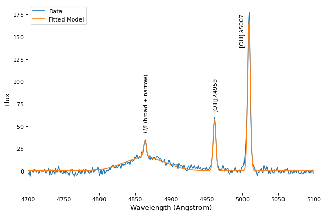
这个 tied 约束通常对以下对象有用 Compound models 。在本例中,我们将从一个名为 spec.txt 并同时将高斯与发射线匹配,同时连接它们的波长和 [OIII] λ4959线路连接到 [OIII] λ5007线。
import numpy as np
from astropy.io import ascii
from astropy.modeling import fitting, models
from astropy.utils.data import get_pkg_data_filename
from matplotlib import pyplot as plt

fname = get_pkg_data_filename("data/spec.txt", package="astropy.modeling.tests")
spec = ascii.read(fname)
wave = spec["lambda"]
flux = spec["flux"]

# Use the (vacuum) rest wavelengths of known lines as initial values
# for the fit.
Hbeta = 4862.721
O3_4959 = 4960.295
O3_5007 = 5008.239

# Create Gaussian1D models for each of the H-beta and [OIII] lines.
hbeta_broad = models.Gaussian1D(amplitude=15, mean=Hbeta, stddev=20)
hbeta_narrow = models.Gaussian1D(amplitude=20, mean=Hbeta, stddev=2)
o3_4959 = models.Gaussian1D(amplitude=70, mean=O3_4959, stddev=2)
o3_5007 = models.Gaussian1D(amplitude=180, mean=O3_5007, stddev=2)

# Create a polynomial model to fit the continuum.
mean_flux = flux.mean()
cont = np.where(flux > mean_flux, mean_flux, flux)
linfitter = fitting.LinearLSQFitter()
poly_cont = linfitter(models.Polynomial1D(1), wave, cont)

# Create a compound model for the four emission lines and the continuum.
model = hbeta_broad + hbeta_narrow + o3_4959 + o3_5007 + poly_cont

# Tie the ratio of the intensity of the two [OIII] lines.
def tie_o3_ampl(model):
    return model.amplitude_3 / 2.98

o3_4959.amplitude.tied = tie_o3_ampl

# Tie the wavelengths of the two [OIII] lines
def tie_o3_wave(model):
    return model.mean_3 * O3_4959 / O3_5007

o3_4959.mean.tied = tie_o3_wave

# Tie the wavelengths of the two (narrow and broad) H-beta lines
def tie_hbeta_wave1(model):
    return model.mean_1

hbeta_broad.mean.tied = tie_hbeta_wave1

# Tie the wavelengths of the H-beta lines to the [OIII] 5007 line
def tie_hbeta_wave2(model):
    return model.mean_3 * Hbeta / O3_5007

hbeta_narrow.mean.tied = tie_hbeta_wave2

# Simultaneously fit all the emission lines and continuum.
fitter = fitting.TRFLSQFitter()
fitted_model = fitter(model, wave, flux)
fitted_lines = fitted_model(wave)

# Plot the data and the fitted model
fig, ax = plt.subplots(figsize=(9, 6))
ax.plot(wave, flux, label="Data")
ax.plot(wave, fitted_lines, color="C1", label="Fitted Model")
ax.legend(loc="upper left")
ax.text(4860, 45, r"$H\beta$ (broad + narrow)", rotation=90)
ax.text(4958, 68, r"[OIII] $\lambda 4959$", rotation=90)
ax.text(4995, 140, r"[OIII] $\lambda 5007$", rotation=90)
ax.set(xlim=(4700, 5100), xlabel="Wavelength (Angstrom)", ylabel="Flux")
plt.show()
