
拟合模型集#
Astropy模型集允许您将同一(线性)模型拟合到大量独立的数据集。它同时求解线性方程组,避免了循环。但是将数据转换成正确的形状可能有点棘手。
节省的时间是值得的。在下面的例子中,如果我们改变宽度 数据立方体的高度为500 500一台2015年的MacBook Pro需要140毫秒才能使用模型集来匹配模型。在500*500型号上循环进行同样的匹配需要1.5分钟,速度慢了600多倍。
在下面的例子中,我们创建了一个三维数据立方体,其中第一个维度是一个斜坡——例如,从红外探测器的非破坏性读数。所以每个像素都有一个沿时间轴的深度,和通量,这会导致计数的总数随时间而增加。我们将拟合1D多项式与时间的关系,以计数/秒(拟合斜率)来估计通量。我们将使用3行4列的小图像,深度为10个非破坏性读取。
首先,导入必要的库:
>>> import numpy as np
>>> rng = np.random.default_rng(seed=12345)
>>> from astropy.modeling import models, fitting
>>> depth, width, height = 10, 3, 4  # Time is along the depth axis
>>> t = np.arange(depth, dtype=np.float64)*10.  # e.g. readouts every 10 seconds
每个像素的计数数是通量*时间加上一些高斯噪声:
>>> fluxes = np.arange(1. * width * height).reshape(width, height)
>>> image = fluxes[np.newaxis, :, :] * t[:, np.newaxis, np.newaxis]
>>> image += rng.normal(0., image*0.05, size=image.shape)  # Add noise
>>> image.shape
(10, 3, 4)
创建模型和装配工。我们需要相同线性参数化模型的N=width*height实例(模型集当前仅适用于线性模型和装配工):
>>> N = width * height
>>> line = models.Polynomial1D(degree=1, n_models=N)
>>> fit = fitting.LinearLSQFitter()
>>> print(f"We created {len(line)} models")
We created 12 models
我们需要使数据符合正确的形状。不可能只给三维数据立方体提供数据。在这种情况下,时间轴可以是一维的。通量必须组织成一个形状的数组 width*height,depth --换言之,我们正在重塑形状,使最后两个轴变平,并将它们放在第一位:
>>> pixels = image.reshape((depth, width*height))
>>> y = pixels.T
>>> print("x axis is one dimensional: ",t.shape)
x axis is one dimensional:  (10,)
>>> print("y axis is two dimensional, N by len(x): ", y.shape)
y axis is two dimensional, N by len(x):  (12, 10)
安装模型。它同时适用于N个模型:
>>> new_model = fit(line, x=t, y=y)
>>> print(f"We fit {len(new_model)} models")
We fit 12 models
使用从最佳拟合计算出的值填充数组,并重新调整其形状以与原始数组匹配:
>>> best_fit = new_model(t, model_set_axis=False).T.reshape((depth, height, width))
>>> print("We reshaped the best fit to dimensions: ", best_fit.shape)
We reshaped the best fit to dimensions:  (10, 4, 3)
现在检查模型:
>>> print(new_model)
Model: Polynomial1D
Inputs: ('x',)
Outputs: ('y',)
Model set size: 12
Degree: 1
Parameters:
             c0                 c1
    ------------------- ------------------
                    0.0                0.0
     0.7435257251672668 0.9788645710692938
    -2.9342067207465647  2.038294797728997
     -4.258776494573452 3.1951399579785678
      2.364390501364263 3.9973270072631104
      2.161531512810536  4.939542306192216
     3.9930177540418823  5.967786182181591
     -6.825657765397985 7.2680615507233215
     -6.675677073701012  8.321048309260679
     -11.91115500400788  9.025794163936956
     -4.123655771677581  9.938564642105128
    -0.7256700167533869 10.989896974949136

>>> print("The new_model has a param_sets attribute with shape: ",new_model.param_sets.shape)
The new_model has a param_sets attribute with shape:  (2, 12)

>>> print(f"And values that are the best-fit parameters for each pixel:\n{new_model.param_sets}")
And values that are the best-fit parameters for each pixel:
[[  0.           0.74352573  -2.93420672  -4.25877649   2.3643905
    2.16153151   3.99301775  -6.82565777  -6.67567707 -11.911155
   -4.12365577  -0.72567002]
 [  0.           0.97886457   2.0382948    3.19513996   3.99732701
    4.93954231   5.96778618   7.26806155   8.32104831   9.02579416
    9.93856464  10.98989697]]
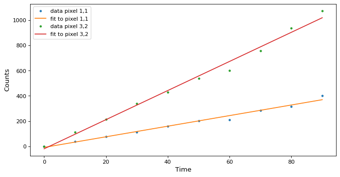
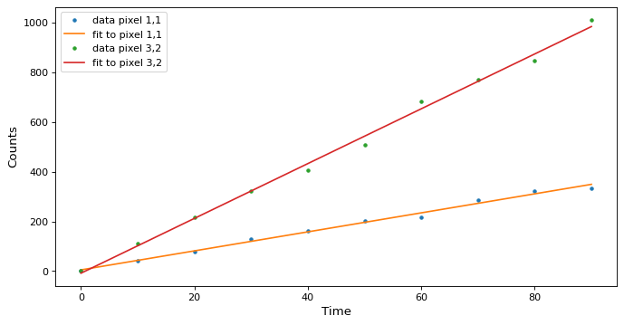
沿几个像素绘制拟合图:
>>> def plotramp(ax, t, image, best_fit, row, col):
...     ax.plot(t, image[:, row, col], '.', label=f'data pixel {row},{col}')
...     ax.plot(t, best_fit[:, row, col], '-', label=f'fit to pixel {row},{col}')
...     ax.set(xlabel='Time', ylabel='Counts')
...     ax.legend(loc='upper left')
>>> fig, ax = plt.subplots(figsize=(10, 5))
>>> plotramp(ax, t, image, best_fit, 1, 1)
>>> plotramp(ax, t, image, best_fit, 2, 1)
数据和最佳拟合模型一起显示在一个图上。