>>> from env_helper import info; info()
页面更新时间: 2024-03-04 14:22:47
运行环境:
    Linux发行版本: Debian GNU/Linux 12 (bookworm)
    操作系统内核: Linux-6.1.0-18-amd64-x86_64-with-glibc2.36
    Python版本: 3.11.2
11.4. 数据处理方法
11.4.1. 几何操作
geopandas在shapely库中提供了所有几何操作的工具。
请注意,所有用于创建不同空间数据集(如创建交叉点或差异)新形状的集合理论工具的文档可以在设置操作页面上查找。
创建方法
GeoSeries.buffer(distance, resolution=16)
返回每个几何对象的给定距离内的所有点的GeoSeries。
GeoSeries.boundary
返回每个几何的集合理论边界的低维对象GeoSeries。
GeoSeries.centroid
返回每个几何质心的点GeoSeries。
GeoSeries.convex_hull
返回包含每个对象所有点的最小凸多边形的几何体的GeoSeries,除非对象中的点数小于三。对于两个点,凸多边形返货的是一个LineString;若为1,则表示一个点。
GeoSeries.envelope
返回包含每个对象点的最小矩形(平行于坐标轴的边)的几何体的GeoSeries。
GeoSeries.simplify(tolerance, preserve_topology=True)
返回包含每个对象简化表示的GeoSeries。
GeoSeries.unary_union
返回包含GeoSeries中所有几何并集的GeoSeries。
仿射变换
GeoSeries.rotate(self, angle, origin='center', use_radians=False)
旋转GeoSeries坐标。
GeoSeries.scale(self, xfact=1.0, yfact=1.0, zfact=1.0, origin='center')
沿每个(x,y,z)维度缩放GeoSeries几何。
GeoSeries.skew(self, angle, origin='center', use_radians=False)
通过沿x和y维度的角度剪切或倾斜GeoSeries的几何图形。
GeoSeries.translate(self, angle, origin='center', use_radians=False)
移动GeoSeries的坐标。
几何操作的示例
>>> %matplotlib inline
>>>
>>> import geopandas as gpd
>>> from geopandas import GeoDataFrame
>>> from shapely.geometry import Polygon
>>> from geopandas import GeoSeries
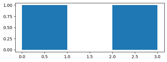
>>> p1 = Polygon([(0, 0), (1, 0), (1, 1)])
>>> p2 = Polygon([(0, 0), (1, 0), (1, 1), (0, 1)])
>>> p3 = Polygon([(2, 0), (3, 0), (3, 1), (2, 1)])
>>> g = GeoSeries([p1, p2, p3])
返回正常的pandas对象。GeoSeries的area属性将返回包含GeoSeries中每个项目的区域的pandas.Series:
>>> print (g.area)
0    0.5
1    1.0
2    1.0
dtype: float64
返回GeoPandas对象:
>>> g.buffer(0.5)
0    POLYGON ((-0.35355 0.35355, 0.64645 1.35355, 0...
1    POLYGON ((-0.50000 0.00000, -0.50000 1.00000, ...
2    POLYGON ((1.50000 0.00000, 1.50000 1.00000, 1....
dtype: geometry
GeoPandas使用的是descartes方法生成matplotlib图。要生成我们自己的GeoSeries图,请使用:
>>> g.plot()
<AxesSubplot: >
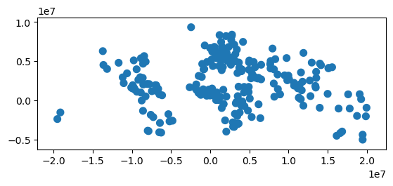
为了演示更复杂的操作,我们将生成一个包含2000个随机点的GeoSeries:
>>> from shapely.geometry import Point
>>> import numpy as np
>>> xmin, xmax, ymin, ymax = 900000, 1080000, 120000, 280000
>>> xc = (xmax - xmin) * np.random.random(2000) + xmin
>>> yc = (ymax - ymin) * np.random.random(2000) + ymin
>>> pts = GeoSeries([Point(x, y) for x, y in zip(xc, yc)])
现在在每个点周围画一个固定半径的圆:
>>> circles = pts.buffer(2000)
我们可以将这些圆形折叠成一个单一的多边形
>>> mp = circles.unary_union
11.4.2. 使用覆盖设置操作
当使用多个空间数据集(尤其是多个多边形或线数据集)时,用户通常想用这些重叠(或不重叠)位置的数据集创建新的形状。这些操作通常使用的是交集集合,通过联合和差异的方法来引用。可通过overlay 函数在geopandas库中操作。
覆盖的DataFrame级别并不是在单个几何体上操作,而是两者的属性都保留。实际上,对于第一个GeoDataFrame中形状来说,此操作针对于其他GeoDataFrame中的每个形状执行:
(熟悉shapely库的用户的请注意:overlay可以被认为是提供标准形状操作的版本,对于处理两个GeoSeries应用集合操作的复杂性来讲,标准的形状集合操作也可以作为GeoSeries方法。)
不同的Overlay操作
首先,我们创建一些示例数据:
>>> from shapely.geometry import Polygon
>>>
>>> polys1 = gpd.GeoSeries([Polygon([(0,0), (2,0), (2,2), (0,2)]),
>>>                        Polygon([(2,2), (4,2), (4,4), (2,4)])])
>>> polys2 = gpd.GeoSeries([Polygon([(1,1), (3,1), (3,3), (1,3)]),
>>>                        Polygon([(3,3), (5,3), (5,5), (3,5)])])
>>> df1 = gpd.GeoDataFrame({'geometry': polys1, 'df1':[1,2]})
>>> df2 = gpd.GeoDataFrame({'geometry': polys2, 'df2':[1,2]})
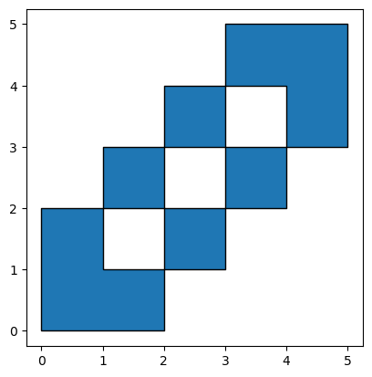
这两个GeoDataFrames有一些重叠区域:
>>> ax = df1.plot(color='red');
>>>
>>> df2.plot(ax=ax, color='green');
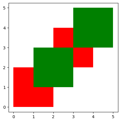
上面的例子说明是的覆盖模式。覆盖函数是通过覆盖GeoDataFrames的方法来确定所有单个几何的集合。此结果覆盖由两个输入GeoDataFrames覆盖的区域组成,保留着两个GeoDataFrames组合边界定义的唯一区域。
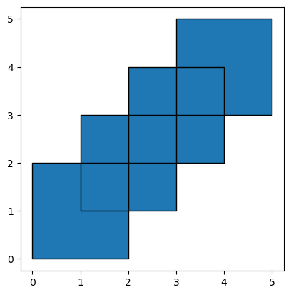
当使用how =’union’时,将返回所有可能的几何体:
>>> res_union = gpd.overlay(df1, df2, how='union')
>>>
>>> res_union
| df1 | df2 | geometry | |
|---|---|---|---|
| 0 | 1.0 | 1.0 | POLYGON ((2.00000 2.00000, 2.00000 1.00000, 1.... |
| 1 | 2.0 | 1.0 | POLYGON ((2.00000 2.00000, 2.00000 3.00000, 3.... |
| 2 | 2.0 | 2.0 | POLYGON ((4.00000 4.00000, 4.00000 3.00000, 3.... |
| 3 | 1.0 | NaN | POLYGON ((2.00000 0.00000, 0.00000 0.00000, 0.... |
| 4 | 2.0 | NaN | MULTIPOLYGON (((3.00000 3.00000, 4.00000 3.000... |
| 5 | NaN | 1.0 | MULTIPOLYGON (((2.00000 2.00000, 3.00000 2.000... |
| 6 | NaN | 2.0 | POLYGON ((3.00000 5.00000, 5.00000 5.00000, 5.... |
>>> ax = res_union.plot()
>>>
>>> df1.plot(ax=ax, facecolor='none');
>>>
>>> df2.plot(ax=ax, facecolor='none');
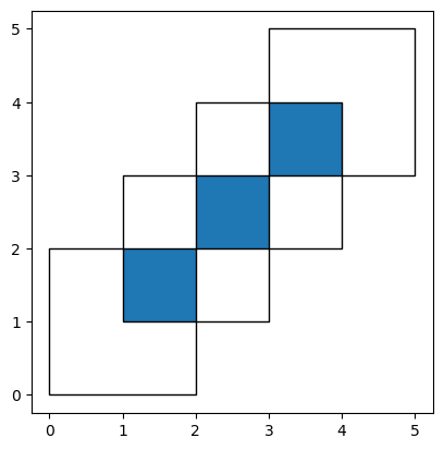
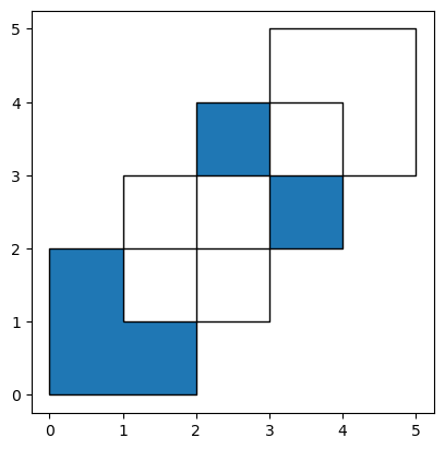
其他操作将返回那些几何的不同子集。使用how =’intersection’方法,返回的是两个GeoDataFrames包含的几何体:
>>> res_intersection = gpd.overlay(df1, df2, how='intersection')
>>>
>>> res_intersection
| df1 | df2 | geometry | |
|---|---|---|---|
| 0 | 1 | 1 | POLYGON ((2.00000 2.00000, 2.00000 1.00000, 1.... |
| 1 | 2 | 1 | POLYGON ((2.00000 2.00000, 2.00000 3.00000, 3.... |
| 2 | 2 | 2 | POLYGON ((4.00000 4.00000, 4.00000 3.00000, 3.... |
>>> ax = res_intersection.plot()
>>>
>>> df1.plot(ax=ax, facecolor='none');
>>>
>>> df2.plot(ax=ax, facecolor='none');
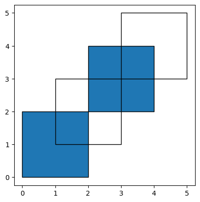
how =’symmetric_difference’与’intersection’相反,返回的几何只是GeoDataFrames其中之一的一部分,并不是两者的一部分:
>>> res_symdiff = gpd.overlay(df1, df2, how='symmetric_difference')
>>>
>>> res_symdiff
| df1 | df2 | geometry | |
|---|---|---|---|
| 0 | 1.0 | NaN | POLYGON ((2.00000 0.00000, 0.00000 0.00000, 0.... |
| 1 | 2.0 | NaN | MULTIPOLYGON (((3.00000 3.00000, 4.00000 3.000... |
| 2 | NaN | 1.0 | MULTIPOLYGON (((2.00000 2.00000, 3.00000 2.000... |
| 3 | NaN | 2.0 | POLYGON ((3.00000 5.00000, 5.00000 5.00000, 5.... |
>>> ax = res_symdiff.plot()
>>>
>>> df1.plot(ax=ax, facecolor='none');
>>>
>>> df2.plot(ax=ax, facecolor='none');
作为df1的一部分但此部分并不包含在df2中,要获取这样的几何体,可以使用how =’difference’方法:
>>> res_difference = gpd.overlay(df1, df2, how='difference')
>>>
>>> res_difference
| geometry | df1 | |
|---|---|---|
| 0 | POLYGON ((2.00000 0.00000, 0.00000 0.00000, 0.... | 1 |
| 1 | MULTIPOLYGON (((3.00000 3.00000, 4.00000 3.000... | 2 |
>>> ax = res_difference.plot()
>>>
>>> df1.plot(ax=ax, facecolor='none');
>>>
>>> df2.plot(ax=ax, facecolor='none');
最后,使用how =’identity’方法生成的,结果由df1的表面组成。若想获得df2覆盖df1的几何体,可使用以下方法:
>>> res_identity = gpd.overlay(df1, df2, how='identity')
>>>
>>> res_identity
| df1 | df2 | geometry | |
|---|---|---|---|
| 0 | 1.0 | 1.0 | POLYGON ((2.00000 2.00000, 2.00000 1.00000, 1.... |
| 1 | 2.0 | 1.0 | POLYGON ((2.00000 2.00000, 2.00000 3.00000, 3.... |
| 2 | 2.0 | 2.0 | POLYGON ((4.00000 4.00000, 4.00000 3.00000, 3.... |
| 3 | 1.0 | NaN | POLYGON ((2.00000 0.00000, 0.00000 0.00000, 0.... |
| 4 | 2.0 | NaN | MULTIPOLYGON (((3.00000 3.00000, 4.00000 3.000... |
>>> ax = res_identity.plot()
>>>
>>> df1.plot(ax=ax, facecolor='none');
>>>
>>> df2.plot(ax=ax, facecolor='none');
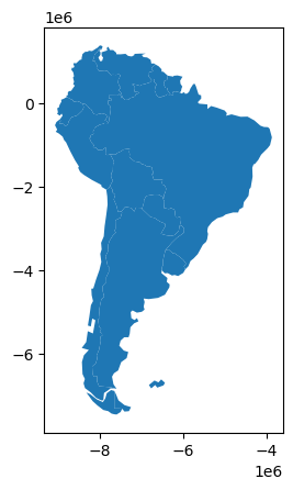
覆盖国家的示例
首先,我们加载国家和城市示例数据集,然后选择:
>>> world = gpd.read_file(gpd.datasets.get_path('naturalearth_lowres'))
>>>
>>> capitals = gpd.read_file(gpd.datasets.get_path('naturalearth_cities'))
>>>
>>> # Select South Amarica and some columns
>>> countries = world[world['continent'] == "South America"]
>>> countries = countries[['geometry', 'name']]
>>>
>>> # Project to crs that uses meters as distance measure
>>> countries = countries.to_crs('epsg:3395')
>>> capitals = capitals.to_crs('epsg:3395')
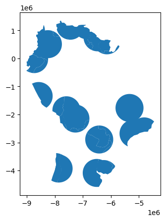
为了说明overlay 功能,我们来假设以下情况,使用国家的GeoDataFrame和大写的GeoDataFrame来识别每个国家的“核心”部分(定义在首都500km内的区域)。
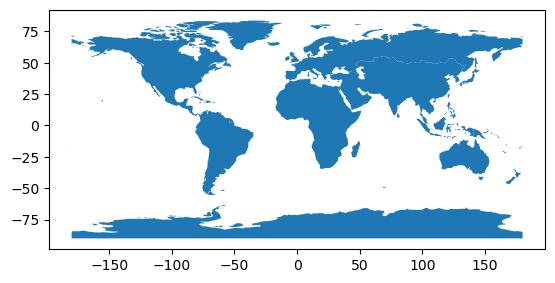
>>> # Look at countries:
>>> countries.plot();
>>>
>>> # Now buffer cities to find area within 500km.
>>> # Check CRS -- World Mercator, units of meters.
>>> capitals.crs
>>>
>>>
>>> # make 500km buffer
>>> capitals['geometry']= capitals.buffer(500000)
>>>
>>> capitals.plot();
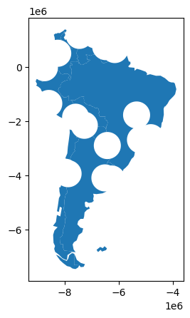
仅选择距离首都500公里内的国家部分,我们指定的如何选项是“intersect”,这将创建一组新的多边形,其中这两个层是重叠的:
>>> country_cores = gpd.overlay(countries, capitals, how='intersection')
>>> country_cores.plot();
更改“方式”选项可允许不同类型的重叠操作。例如,我们对远离国家首都的部分感兴趣,可以计算两者的差异。
>>> country_peripheries = gpd.overlay(countries, capitals, how='difference')
>>> country_peripheries.plot();
11.4.3. 要素融合
通常情况下,我们发现自己使用的空间数据比我们需要的粒度更细。例如,我们有国家地方单位的数据,但我们感兴趣的是研究国家层面的模式。
在非空间设置中,我们使用groupby函数聚合数据。但是使用空间数据时,可能会需要一个特殊的工具,也可以聚合几何特征。在geopandas库中,该功能由dissolve函数提供。
dissolve可以做三件事情:(a)它将给定组中的所有几何图形,并一起溶解成单个几何特征(使用unary_union方法);(b)它聚合组中的所有数据行,使用的是groupby.aggregate()方法;(c)将以上这两种方法结合。
dissolve示例
假设我们对研究大陆感兴趣,但我们只有国家级数据。我们可以轻松地将其转换为大陆级数据集。
首先,我们只需要大陆形状和名称。默认情况下,dissolve将’first’输出到groupby.aggregate。
>>> world = gpd.read_file(gpd.datasets.get_path('naturalearth_lowres'))
>>>
>>> world = world[['continent', 'geometry']]
>>>
>>> continents = world.dissolve(by='continent')
>>>
>>> continents.plot();
>>>
>>> continents.head()
| geometry | |
|---|---|
| continent | |
| Africa | MULTIPOLYGON (((-11.43878 6.78592, -11.70819 6... |
| Antarctica | MULTIPOLYGON (((-61.13898 -79.98137, -60.61012... |
| Asia | MULTIPOLYGON (((48.67923 14.00320, 48.23895 13... |
| Europe | MULTIPOLYGON (((-53.55484 2.33490, -53.77852 2... |
| North America | MULTIPOLYGON (((-155.22217 19.23972, -155.5421... |
11.4.4. 合并数据
有两种方法可以合并地理数据库中数据集中的属性连接和空间连接。
在属性连接中,GeoSeries或GeoDataFrame与基于常见变量的常规pandas Series或DataFrame组合。有类似于普通合并或加入pandas。
在空间连接中,由于GeoSeries与GeoDataFrames彼此的空间关系而被组合。
在下面的示例中,我们使用这些数据集:
>>> %matplotlib inline
>>> import geopandas as gpd
>>>
>>> world = gpd.read_file(gpd.datasets.get_path('naturalearth_lowres'))
>>>
>>> cities = gpd.read_file(gpd.datasets.get_path('naturalearth_cities'))
>>>
>>> # For attribute join
>>> country_shapes = world[['geometry', 'iso_a3']]
>>>
>>> country_names = world[['name', 'iso_a3']]
>>>
>>> # For spatial join
>>> countries = world[['geometry', 'name']]
>>>
>>> countries = countries.rename(columns={'name':'country'})
属性连接
属性连接可使用merge方法完成。通常,建议使用空间数据集调用merge的方法。如果GeoDataFrame在left参数中,merge函数将独立工作;如果DataFrame在left参数中,并且GeoDataFrame在right的位置,那么结果将不再是GeoDataFrame。
通过与pandas DataFrame合并,为GeoDataFrame添加全名的方法,该GeoDataFrame会具有每个国家/地区的ISO代码。
>>> # country_shapes` is GeoDataFrame with country shapes and iso codes
>>>
>>> country_shapes.head()
| geometry | iso_a3 | |
|---|---|---|
| 0 | MULTIPOLYGON (((180.00000 -16.06713, 180.00000... | FJI |
| 1 | POLYGON ((33.90371 -0.95000, 34.07262 -1.05982... | TZA |
| 2 | POLYGON ((-8.66559 27.65643, -8.66512 27.58948... | ESH |
| 3 | MULTIPOLYGON (((-122.84000 49.00000, -122.9742... | CAN |
| 4 | MULTIPOLYGON (((-122.84000 49.00000, -120.0000... | USA |
>>> country_names.head()
| name | iso_a3 | |
|---|---|---|
| 0 | Fiji | FJI |
| 1 | Tanzania | TZA |
| 2 | W. Sahara | ESH |
| 3 | Canada | CAN |
| 4 | United States of America | USA |
>>> country_shapes = country_shapes.merge(country_names, on='iso_a3')
>>>
>>> country_shapes.head()
| geometry | iso_a3 | name | |
|---|---|---|---|
| 0 | MULTIPOLYGON (((180.00000 -16.06713, 180.00000... | FJI | Fiji |
| 1 | POLYGON ((33.90371 -0.95000, 34.07262 -1.05982... | TZA | Tanzania |
| 2 | POLYGON ((-8.66559 27.65643, -8.66512 27.58948... | ESH | W. Sahara |
| 3 | MULTIPOLYGON (((-122.84000 49.00000, -122.9742... | CAN | Canada |
| 4 | MULTIPOLYGON (((-122.84000 49.00000, -120.0000... | USA | United States of America |
空间连接
在空间联接中,两个几何对象基于它们彼此的空间关系而被合并。
>>> # One GeoDataFrame of countries, one of Cities.
>>> # Want to merge so we can get each city's country.
>>> countries.head()
| geometry | country | |
|---|---|---|
| 0 | MULTIPOLYGON (((180.00000 -16.06713, 180.00000... | Fiji |
| 1 | POLYGON ((33.90371 -0.95000, 34.07262 -1.05982... | Tanzania |
| 2 | POLYGON ((-8.66559 27.65643, -8.66512 27.58948... | W. Sahara |
| 3 | MULTIPOLYGON (((-122.84000 49.00000, -122.9742... | Canada |
| 4 | MULTIPOLYGON (((-122.84000 49.00000, -120.0000... | United States of America |
>>> cities.head()
| name | geometry | |
|---|---|---|
| 0 | Vatican City | POINT (12.45339 41.90328) |
| 1 | San Marino | POINT (12.44177 43.93610) |
| 2 | Vaduz | POINT (9.51667 47.13372) |
| 3 | Lobamba | POINT (31.20000 -26.46667) |
| 4 | Luxembourg | POINT (6.13000 49.61166) |
>>> cities_with_country = gpd.sjoin(cities, countries, how="inner", predicate='intersects')
>>>
>>> cities_with_country.head()
| name | geometry | index_right | country | |
|---|---|---|---|---|
| 0 | Vatican City | POINT (12.45339 41.90328) | 141 | Italy |
| 1 | San Marino | POINT (12.44177 43.93610) | 141 | Italy |
| 226 | Rome | POINT (12.48131 41.89790) | 141 | Italy |
| 2 | Vaduz | POINT (9.51667 47.13372) | 114 | Austria |
| 212 | Vienna | POINT (16.36469 48.20196) | 114 | Austria |