>>> from env_helper import info; info()
页面更新时间: 2023-12-24 17:20:20
运行环境:
    Linux发行版本: Debian GNU/Linux 12 (bookworm)
    操作系统内核: Linux-6.1.0-15-amd64-x86_64-with-glibc2.36
    Python版本: 3.11.2
10.5. Cartopy地图绘图2
这里展示两个例子。可以用于地图学教学中。
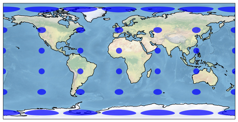
10.5.1. Tissot’s indicatrix
法国数学家 Nicolas Auguste Tissot 于 1859 年提出Tissot indicatrix 图用于表征地图投影的畸变特性。
在地图上显示Tissot’s indicatrix
>>> import matplotlib.pyplot as plt
>>>
>>> import cartopy.crs as ccrs
>>>
>>> fig = plt.figure(figsize=(10, 5))
>>> ax = fig.add_subplot(1, 1, 1, projection=ccrs.PlateCarree())
>>>
>>> # make the map global rather than have it zoom in to
>>> # the extents of any plotted data
>>> ax.set_global()
>>>
>>> ax.stock_img()
>>> ax.coastlines()
>>>
>>> ax.tissot(facecolor='blue', alpha=0.7)
>>>
>>> plt.show()
/usr/lib/python3/dist-packages/cartopy/mpl/geoaxes.py:801: UserWarning: Approximating coordinate system <Geographic 2D CRS: +proj=lonlat +datum=WGS84 +ellps=WGS84 +no_defs +t ...>
Name: unknown
Axis Info [ellipsoidal]:
- lon[east]: Longitude (degree)
- lat[north]: Latitude (degree)
Area of Use:
- undefined
Datum: World Geodetic System 1984
- Ellipsoid: WGS 84
- Prime Meridian: Greenwich
 with the PlateCarree projection.
  warnings.warn(f'Approximating coordinate system {crs!r} with '
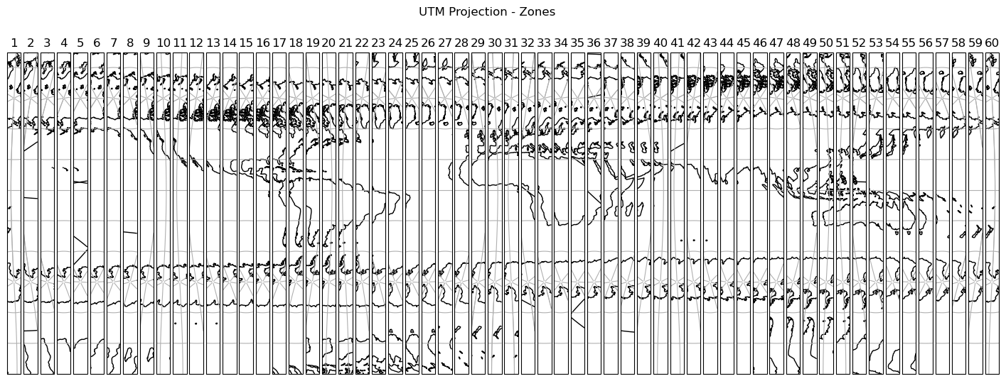
10.5.2. 显示UTM投影的所有60个区域
本例以图形的形式显示了通用横轴墨卡托投影的所有60个区域。 首先我们创建一个一行有60个子块的图。接下来,我们将图中的每个轴投影到一个特定的UTM区域。然后我们添加海岸线、网格线和区域编号。最后,我们添加一个超级标题并显示图形。
>>> import cartopy.crs as ccrs
>>> import matplotlib.pyplot as plt
>>>
>>>
>>>
>>> # Create a list of integers from 1 - 60
>>> zones = range(1, 61)
>>>
>>> # Create a figure
>>> fig = plt.figure(figsize=(18, 6))
>>>
>>> # Loop through each zone in the list
>>> for zone in zones:
>>>
>>>     # Add GeoAxes object with specific UTM zone projection to the figure
>>>     ax = fig.add_subplot(
>>>         1, len(zones), zone,
>>>         projection=ccrs.UTM(
>>>             zone=zone,
>>>             southern_hemisphere=True
>>>         )
>>>     )
>>>
>>>     # Add coastlines, gridlines and zone number for the subplot
>>>     ax.coastlines(resolution='110m')
>>>     ax.gridlines()
>>>     ax.set_title(zone)
>>>
>>> # Add a supertitle for the figure
>>> fig.suptitle("UTM Projection - Zones")
>>>
>>> # Display the figure
>>> plt.show()