>>> from env_helper import info; info()
页面更新时间: 2023-12-24 17:19:43
运行环境:
    Linux发行版本: Debian GNU/Linux 12 (bookworm)
    操作系统内核: Linux-6.1.0-15-amd64-x86_64-with-glibc2.36
    Python版本: 3.11.2
10.3. Cartopy绘图功能
10.3.1. 在cartopy中修改地图的边界
此示例演示如何修改地图的边界。我们在 PlateCarree 坐标系中构造一个有坐标的五角星,并用它作为地图的轮廓。 请注意,更改地图的投影如何表示投影的星形边界。
Construct a star in longitudes and latitudes.
>>> import matplotlib.path as mpath
>>> star_path = mpath.Path.unit_regular_star(5, 0.5)
>>> star_path = mpath.Path(
>>>     star_path.vertices.copy() * 80,
>>>     star_path.codes.copy()
>>> )
Use the star as the boundary.
>>> import matplotlib.pyplot as plt
>>> import cartopy.crs as ccrs
>>> fig = plt.figure()
>>> ax = fig.add_axes([0, 0, 1, 1], projection=ccrs.PlateCarree())
>>> ax.coastlines()
>>> ax.set_boundary(star_path, transform=ccrs.PlateCarree())
>>> plt.show()

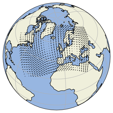
10.3.2. 箭头
绘制箭头。
>>> import matplotlib.pyplot as plt
>>> import numpy as np
>>>
>>> import cartopy.crs as ccrs
>>> import cartopy.feature as cfeature
>>>
>>>
>>> def sample_data(shape=(20, 30)):
>>>     """
>>>     Return ``(x, y, u, v, crs)`` of some vector data
>>>     computed mathematically. The returned crs will be a rotated
>>>     pole CRS, meaning that the vectors will be unevenly spaced in
>>>     regular PlateCarree space.
>>>
>>>     """
>>>     crs = ccrs.RotatedPole(pole_longitude=177.5, pole_latitude=37.5)
>>>
>>>     x = np.linspace(311.9, 391.1, shape[1])
>>>     y = np.linspace(-23.6, 24.8, shape[0])
>>>
>>>     x2d, y2d = np.meshgrid(x, y)
>>>     u = 10 * (2 * np.cos(2 * np.deg2rad(x2d) + 3 * np.deg2rad(y2d + 30)) ** 2)
>>>     v = 20 * np.cos(6 * np.deg2rad(x2d))
>>>
>>>     return x, y, u, v, crs
>>>
>>>
>>>
>>> fig = plt.figure()
>>> ax = fig.add_subplot(1, 1, 1, projection=ccrs.Orthographic(-10, 45))
>>>
>>> ax.add_feature(cfeature.OCEAN, zorder=0)
>>> ax.add_feature(cfeature.LAND, zorder=0, edgecolor='black')
>>>
>>> ax.set_global()
>>> ax.gridlines()
>>>
>>> x, y, u, v, vector_crs = sample_data()
>>> ax.quiver(x, y, u, v, transform=vector_crs)
>>>
>>> plt.show()
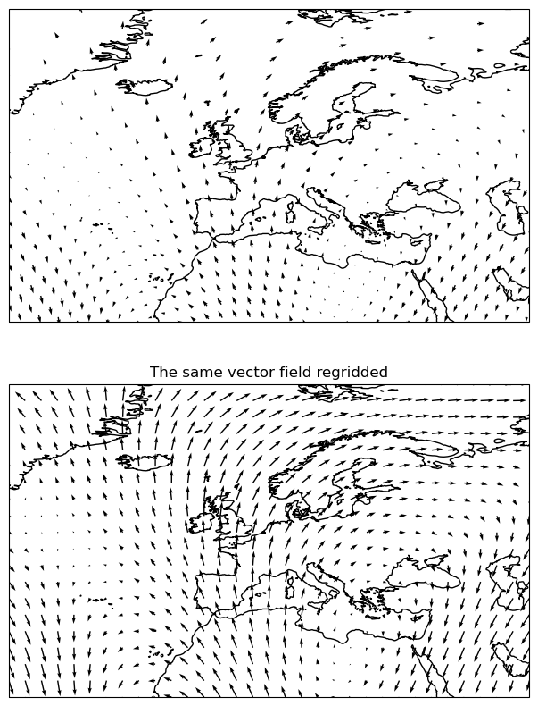
10.3.3. 带抖动的向量重拼接
这个示例演示了在箭头中的重排功能(在
cartopy.mpl.geoaxes.GeoAxes.barbs() 中存在等价的功能。)
重新划分网格是可视化向量场的有效方法,特别是在数据密集或扭曲的情况下。
>>> import matplotlib.pyplot as plt
>>> import numpy as np
>>>
>>> import cartopy.crs as ccrs
>>>
>>>
>>> def sample_data(shape=(20, 30)):
>>>     """
>>>     Return ``(x, y, u, v, crs)`` of some vector data
>>>     computed mathematically. The returned CRS will be a North Polar
>>>     Stereographic projection, meaning that the vectors will be unevenly
>>>     spaced in a PlateCarree projection.
>>>
>>>     """
>>>     crs = ccrs.NorthPolarStereo()
>>>     scale = 1e7
>>>     x = np.linspace(-scale, scale, shape[1])
>>>     y = np.linspace(-scale, scale, shape[0])
>>>
>>>     x2d, y2d = np.meshgrid(x, y)
>>>     u = 10 * np.cos(2 * x2d / scale + 3 * y2d / scale)
>>>     v = 20 * np.cos(6 * x2d / scale)
>>>
>>>     return x, y, u, v, crs
>>>
>>>
>>> fig = plt.figure(figsize=(8, 10))
>>>
>>> x, y, u, v, vector_crs = sample_data(shape=(50, 50))
>>> ax1 = fig.add_subplot(2, 1, 1, projection=ccrs.PlateCarree())
>>> ax1.coastlines('50m')
>>> ax1.set_extent([-45, 55, 20, 80], ccrs.PlateCarree())
>>> ax1.quiver(x, y, u, v, transform=vector_crs)
>>>
>>> ax2 = fig.add_subplot(2, 1, 2, projection=ccrs.PlateCarree())
>>> ax2.set_title('The same vector field regridded')
>>> ax2.coastlines('50m')
>>> ax2.set_extent([-45, 55, 20, 80], ccrs.PlateCarree())
>>> ax2.quiver(x, y, u, v, transform=vector_crs, regrid_shape=20)
>>>
>>> plt.show()
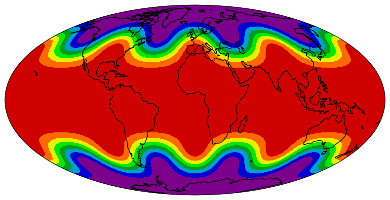
10.3.4. 填充轮廓
制造数据上的轮廓线示例。
>>> import matplotlib.pyplot as plt
>>> import numpy as np
>>>
>>> import cartopy.crs as ccrs
>>>
>>>
>>> def sample_data(shape=(73, 145)):
>>>     """Return ``lons``, ``lats`` and ``data`` of some fake data."""
>>>     nlats, nlons = shape
>>>     lats = np.linspace(-np.pi / 2, np.pi / 2, nlats)
>>>     lons = np.linspace(0, 2 * np.pi, nlons)
>>>     lons, lats = np.meshgrid(lons, lats)
>>>     wave = 0.75 * (np.sin(2 * lats) ** 8) * np.cos(4 * lons)
>>>     mean = 0.5 * np.cos(2 * lats) * ((np.sin(2 * lats)) ** 2 + 2)
>>>
>>>     lats = np.rad2deg(lats)
>>>     lons = np.rad2deg(lons)
>>>     data = wave + mean
>>>
>>>     return lons, lats, data
>>>
>>> fig = plt.figure(figsize=(10, 5))
>>> ax = fig.add_subplot(1, 1, 1, projection=ccrs.Mollweide())
>>>
>>> lons, lats, data = sample_data()
>>>
>>> ax.contourf(lons, lats, data,
>>>             transform=ccrs.PlateCarree(),
>>>             cmap='nipy_spectral')
>>> ax.coastlines()
>>> ax.set_global()
>>> plt.show()