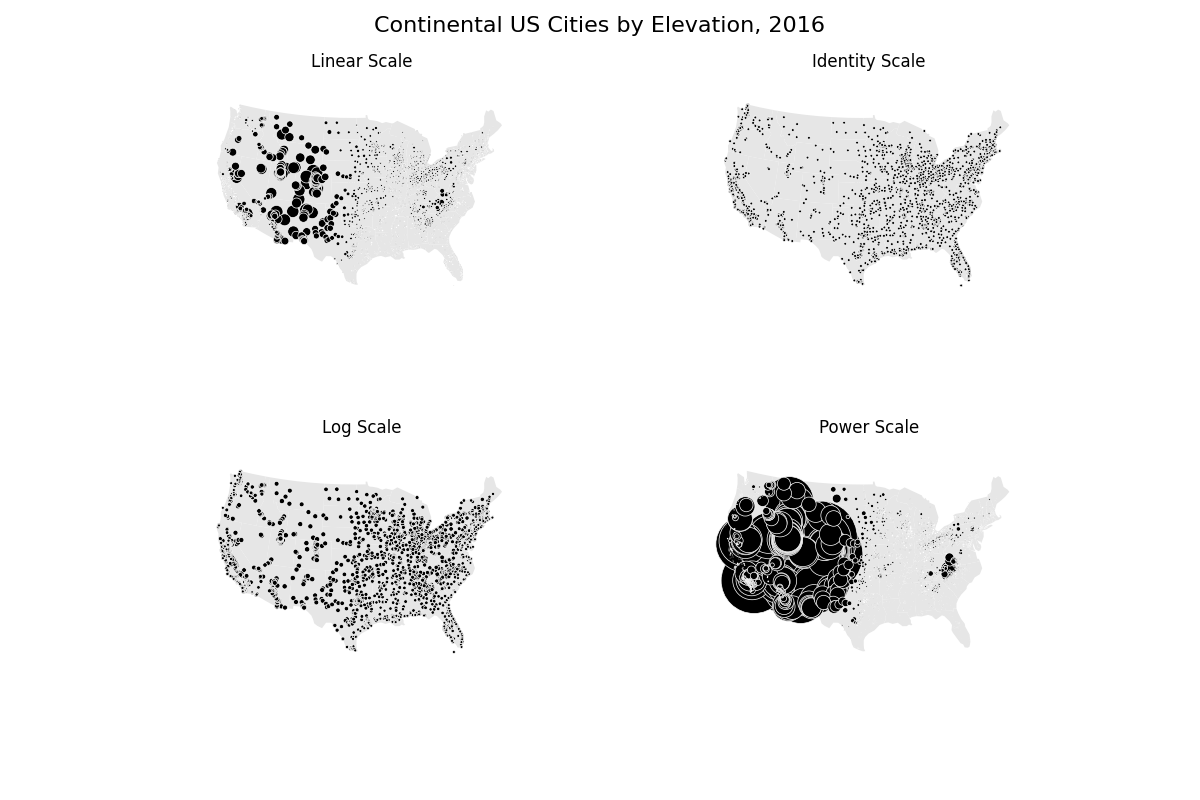
具有自定义比例函数的美国城市高程点图

本例按美国城市的海拔高度绘制城市图。几个不同的可能的标度函数确定点的大小演示。

第一个图是默认的线性比例图。从结果中我们可以看出，这显然是最适合这个具体数据的一个。

第二个图显示了一个微不足道的身份尺度。这样一来，每个城市的面积都是一样的。

一个更有趣的尺度是对数尺度。当所讨论的数据是对数线性的，也就是说，它相对于它自己的对数呈线性分布时，这个比例非常有效。在我们的演示案例中，数据是线性的，在形状上不是logorithm的，所以这个结果不是很好，但在其他情况下，使用logorithm是一种方法。

最后一个演示展示了一个功率秤。这对于遵循某种幂律分布的数据很有用。再说一次，这在我们的案例中并不太有效。

import geopandas as gpd
import geoplot as gplt
import geoplot.crs as gcrs
import numpy as np
import matplotlib.pyplot as plt

continental_usa_cities = gpd.read_file(gplt.datasets.get_path('usa_cities'))
continental_usa_cities = continental_usa_cities.query('STATE not in ["AK", "HI", "PR"]')
contiguous_usa = gpd.read_file(gplt.datasets.get_path('contiguous_usa'))


proj = gcrs.AlbersEqualArea(central_longitude=-98, central_latitude=39.5)
f, axarr = plt.subplots(2, 2, figsize=(12, 8), subplot_kw={'projection': proj})

polyplot_kwargs = {'facecolor': (0.9, 0.9, 0.9), 'linewidth': 0}
pointplot_kwargs = {
    'scale': 'ELEV_IN_FT', 'edgecolor': 'white', 'linewidth': 0.5, 'color': 'black'
}


gplt.polyplot(contiguous_usa.geometry, ax=axarr[0][0], **polyplot_kwargs)
gplt.pointplot(
    continental_usa_cities.query("POP_2010 > 10000"),
    ax=axarr[0][0], limits=(0.1, 10), **pointplot_kwargs
)
axarr[0][0].set_title("Linear Scale")


def identity_scale(minval, maxval):
    def scalar(val):
        return 2
    return scalar

gplt.polyplot(contiguous_usa.geometry, ax=axarr[0][1], **polyplot_kwargs)
gplt.pointplot(
    continental_usa_cities.query("POP_2010 > 10000"),
    ax=axarr[0][1], scale_func=identity_scale, **pointplot_kwargs
)
axarr[0][1].set_title("Identity Scale")


def log_scale(minval, maxval):
    def scalar(val):
        val = val + abs(minval) + 1
        return np.log10(val)
    return scalar

gplt.polyplot(
    contiguous_usa.geometry,
    ax=axarr[1][0], **polyplot_kwargs
)
gplt.pointplot(
    continental_usa_cities.query("POP_2010 > 10000"),
    ax=axarr[1][0], scale_func=log_scale, **pointplot_kwargs
)
axarr[1][0].set_title("Log Scale")


def power_scale(minval, maxval):
    def scalar(val):
        val = val + abs(minval) + 1
        return (val/1000)**2
    return scalar

gplt.polyplot(
    contiguous_usa.geometry,
    ax=axarr[1][1], **polyplot_kwargs
)
gplt.pointplot(
    continental_usa_cities.query("POP_2010 > 10000"),
    ax=axarr[1][1], scale_func=power_scale, **pointplot_kwargs
)
axarr[1][1].set_title("Power Scale")

plt.suptitle('Continental US Cities by Elevation, 2016', fontsize=16)

plt.subplots_adjust(top=0.95)
plt.savefig("usa-city-elevations.png", bbox_inches='tight')