

选择直方图箱#
这个 astropy.visualization 模块提供 hist() 函数,它是matplotlib的直方图函数的一个泛化,它允许更灵活地指定直方图箱。有关不带随附绘图的计算容器,请参见 astropy.stats.histogram() .
为此,考虑以下两个柱状图,它们是从5000个点的同一个基本集合中构造的,第一个柱状图使用matplotlib的默认值10个箱子,第二个柱状图具有任意选择的200个箱子:
import numpy as np
import matplotlib.pyplot as plt

# generate some complicated data
rng = np.random.default_rng(0)
t = np.concatenate([-5 + 1.8 * rng.standard_cauchy(500),
                    -4 + 0.8 * rng.standard_cauchy(2000),
                    -1 + 0.3 * rng.standard_cauchy(500),
                    2 + 0.8 * rng.standard_cauchy(1000),
                    4 + 1.5 * rng.standard_cauchy(1000)])

# truncate to a reasonable range
t = t[(t > -15) & (t < 15)]

# draw histograms with two different bin widths
fig, ax = plt.subplots(1, 2, figsize=(10, 4))

fig.subplots_adjust(left=0.1, right=0.95, bottom=0.15)
for i, bins in enumerate([10, 200]):
    ax[i].hist(t, bins=bins, histtype='stepfilled', alpha=0.2, density=True)
    ax[i].set_xlabel('t')
    ax[i].set_ylabel('P(t)')
    ax[i].set_title(f'plt.hist(t, bins={bins})',
                    fontdict=dict(family='monospace'))
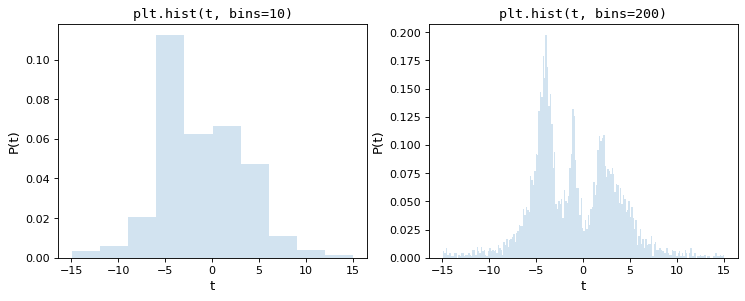
通过目测,很明显这些选择都是次优的:10个仓,数据分布的精细结构丢失,而200个仓,单个仓的高度受取样误差影响。大多数科学家所采用的久经考验的方法是一种尝试和错误的方法,试图在这两者之间找到一个合适的中点。
Astropy的 hist() 函数通过提供几种自动调整直方图箱大小的方法来解决这一问题。它的语法与matplotlib的语法相同 plt.hist 函数,除了 bins 参数,允许指定四种不同方法中的一种来自动选择纸盒。这些方法在中实现 astropy.stats.histogram() ,其语法与 np.histogram 功能。
正常参考规则#
调整存储箱数量的最简单方法是由Scott(在中实现)提供的普通引用规则 scott_bin_width() )和Freedman&Diaconis(在 freedman_bin_width() ). 这些规则通过假设数据接近正态分布,并应用一个经验法则,旨在最小化直方图和数据的基本分布之间的差异。
下图显示了这两个规则对上述数据集的结果:
import numpy as np
import matplotlib.pyplot as plt
from astropy.visualization import hist

# generate some complicated data
rng = np.random.default_rng(0)
t = np.concatenate([-5 + 1.8 * rng.standard_cauchy(500),
                    -4 + 0.8 * rng.standard_cauchy(2000),
                    -1 + 0.3 * rng.standard_cauchy(500),
                    2 + 0.8 * rng.standard_cauchy(1000),
                    4 + 1.5 * rng.standard_cauchy(1000)])

# truncate to a reasonable range
t = t[(t > -15) & (t < 15)]

# draw histograms with two different bin widths
fig, ax = plt.subplots(1, 2, figsize=(10, 4))

fig.subplots_adjust(left=0.1, right=0.95, bottom=0.15)
for i, bins in enumerate(['scott', 'freedman']):
    hist(t, bins=bins, ax=ax[i], histtype='stepfilled',
         alpha=0.2, density=True)
    ax[i].set_xlabel('t')
    ax[i].set_ylabel('P(t)')
    ax[i].set_title(f'hist(t, bins="{bins}")',
                    fontdict=dict(family='monospace'))
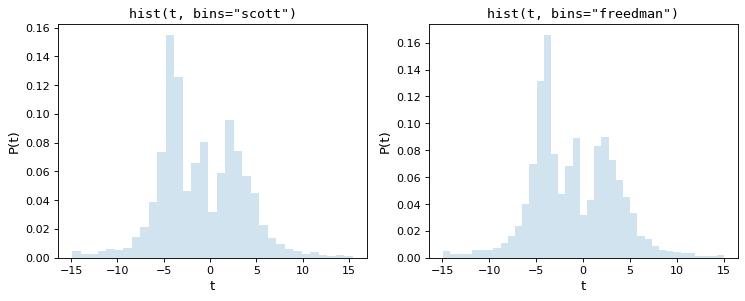
如我们所见,这两个经验法则都选择了中间数量的存储单元,这在数据表示和噪声抑制之间提供了很好的折衷。
贝叶斯模型#
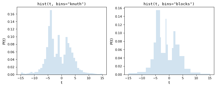
虽然经验法则,如斯科特规则和弗里德曼迪亚康尼斯规则是快速和方便的,但他们对数据的强大假设使其在更复杂的分布中处于次优状态。其他的箱位选择方法使用根据实际数据计算的适应度函数来选择最佳的装箱。Astropy实现了以下两个示例:Knuth规则(在 knuth_bin_width() )和贝叶斯块(在 bayesian_blocks() )
Knuth规则选择一个恒定的数据元大小,最大限度地减少直方图对数据的近似误差,而贝叶斯块则使用一种更灵活的方法,允许改变库宽度。因为这两种方法都要求在整个数据集中最小化成本函数,所以它们比上面提到的经验法则计算量更大。以下是上述数据集的这些程序的结果:
import warnings
import numpy as np
import matplotlib.pyplot as plt
from astropy.visualization import hist

# generate some complicated data
rng = np.random.default_rng(0)
t = np.concatenate([-5 + 1.8 * rng.standard_cauchy(500),
                    -4 + 0.8 * rng.standard_cauchy(2000),
                    -1 + 0.3 * rng.standard_cauchy(500),
                    2 + 0.8 * rng.standard_cauchy(1000),
                    4 + 1.5 * rng.standard_cauchy(1000)])

# truncate to a reasonable range
t = t[(t > -15) & (t < 15)]

# draw histograms with two different bin widths
fig, ax = plt.subplots(1, 2, figsize=(10, 4))

fig.subplots_adjust(left=0.1, right=0.95, bottom=0.15)
for i, bins in enumerate(['knuth', 'blocks']):
    hist(t, bins=bins, ax=ax[i], histtype='stepfilled',
            alpha=0.2, density=True)
    ax[i].set_xlabel('t')
    ax[i].set_ylabel('P(t)')
    ax[i].set_title(f'hist(t, bins="{bins}")',
                    fontdict=dict(family='monospace'))

请注意,这两种方法都非常准确地捕捉了分布的形状,并且 bins='blocks' 面板选择宽度随数据中的局部结构而变化的库宽度。与标准默认值相比,这些贝叶斯优化方法提供了一种更原则的方法来选择直方图分块。