

图像拉伸和归一化#
这个 astropy.visualization 模块提供了一个框架来转换图像中的值(通常是任何数组),通常是为了可视化的目的。提供了两种主要类型的转换:
规范化到 [0:1] 使用下限和上限的范围,其中 \(x\) 表示原始图像中的值:
拉伸 中的值 [0:1] 范围到 [0:1] 使用线性或非线性函数的范围:
此外,还提供了类,以便根据特定算法(例如使用百分位)来确定数据集的上限和下限。
中描述了识别下限和上限以及重新规范化 Intervals and Normalization 第节中介绍了拉伸过程 Stretching 部分。
区间和标准化#
捷径#
astropy 提供了方便 simple_norm() 功能和 SimpleNorm 对于快速交互分析很有用的类。这些便利工具创建了一个 ImageNormalize 规范化对象,可以与Matplotlib的 imshow() 方法
这是一个使用 simple_norm() 功能:
import numpy as np
import matplotlib.pyplot as plt
from astropy.visualization import simple_norm
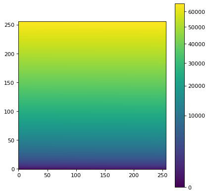
# Generate a test image
image = np.arange(65536).reshape((256, 256))
# Create an ImageNormalize object
norm = simple_norm(image, 'sqrt')
# Display the image
fig, ax = plt.subplots()
im = ax.imshow(image, origin='lower', norm=norm)
fig.colorbar(im)
这是一个使用 SimpleNorm 班级及其 imshow() 方法:
import numpy as np
import matplotlib.pyplot as plt
from astropy.visualization import SimpleNorm

# Generate a test image
image = np.arange(65536).reshape((256, 256))

# Create an ImageNormalize object
snorm = SimpleNorm('sqrt', percent=98)

# Display the image
fig, ax = plt.subplots()
axim = snorm.imshow(image, ax=ax, origin='lower')
fig.colorbar(axim)

详细的方法#
提供了几个类来确定间隔并将此间隔中的值规范化为 [0:1] 范围。最简单的例子之一是 MinMaxInterval 它根据数组中的最小值和最大值确定值的限制。该类没有参数实例化:
>>> from astropy.visualization import MinMaxInterval
>>> interval = MinMaxInterval()
可以通过调用 get_limits() 方法,它采用值数组::
>>> interval.get_limits([1, 3, 4, 5, 6])
(np.int64(1), np.int64(6))
这个 interval 实例也可以像函数一样调用,以实际将值规范化为以下范围:
>>> interval([1, 3, 4, 5, 6])
array([0. , 0.4, 0.6, 0.8, 1. ])
其他间隔类包括 ManualInterval , PercentileInterval , AsymmetricPercentileInterval 和 ZScaleInterval . 对于这些,数组中的值可能超出间隔给定的限制。A clip 参数用于控制值超出限制时规范化的行为:
>>> from astropy.visualization import PercentileInterval
>>> interval = PercentileInterval(50.)
>>> interval.get_limits([1, 3, 4, 5, 6])
(np.float64(3.0), np.float64(5.0))
>>> interval([1, 3, 4, 5, 6])  # default is clip=True
array([0. , 0. , 0.5, 1. , 1. ])
>>> interval([1, 3, 4, 5, 6], clip=False)
array([-1. ,  0. ,  0.5,  1. ,  1.5])
拉伸#
除了可以将值缩放到 [0:1] 范围内,提供了许多类来使用不同的函数“拉伸”值。这些地图 [0:1] 变换后的 [0:1] 范围。一个简单的例子是 SqrtStretch 班级:
>>> from astropy.visualization import SqrtStretch
>>> stretch = SqrtStretch()
>>> stretch([0., 0.25, 0.5, 0.75, 1.])
array([0.        , 0.5       , 0.70710678, 0.8660254 , 1.        ])
至于间隔,值在 [0:1] 根据 clip 争论。默认情况下,输出值被剪裁到 [0:1] 范围:
>>> stretch([-1., 0., 0.5, 1., 1.5])
array([0.       , 0.        , 0.70710678, 1.        , 1.        ])
但可以禁用:
>>> stretch([-1., 0., 0.5, 1., 1.5], clip=False)
array([       nan, 0.        , 0.70710678, 1.        , 1.22474487])
备注
拉伸函数与例如。 DS9 (尽管他们应该有相同的行为)。可以找到DS9拉伸的方程式 here 可以与 astropy.visualization API部分。我们的拉伸和DS9的主要区别在于我们调整了它们,以便 [0:1] 范围始终精确映射到 [0:1] 范围。
组合变换#
任何间隔和延伸都可以通过使用 + 运算符,返回新的转换。组合间隔和拉伸时,拉伸对象必须在间隔对象之前。例如,要基于百分位值和平方根拉伸应用规格化,可以执行以下操作:
>>> transform = SqrtStretch() + PercentileInterval(90.)
>>> transform([1, 3, 4, 5, 6])
array([0.        , 0.60302269, 0.76870611, 0.90453403, 1.        ])
与以前一样,组合转换也可以接受 clip 参数(即 True 默认情况下)。
Matplotlib规范化#
Matplotlib允许在通过传递 matplotlib.colors.Normalize 对象,例如 imshow() . 这个 astropy.visualization module provides an ImageNormalize class that wraps the interval (see Intervals and Normalization )和伸展(参见 Stretching )对象放入Matplotlib理解的对象中。
的输入 ImageNormalize 类是数据和间隔和拉伸对象:
import numpy as np
import matplotlib.pyplot as plt

from astropy.visualization import (MinMaxInterval, SqrtStretch,
                                   ImageNormalize)

# Generate a test image
image = np.arange(65536).reshape((256, 256))

# Create an ImageNormalize object
norm = ImageNormalize(image, interval=MinMaxInterval(),
                      stretch=SqrtStretch())

# or equivalently using positional arguments
# norm = ImageNormalize(image, MinMaxInterval(), SqrtStretch())

# Display the image
fig, ax = plt.subplots()
im = ax.imshow(image, origin='lower', norm=norm)
fig.colorbar(im)

如上所示,colorbar刻度将自动调整。
请注意不要使用 ax.imshow(norm(image)) 因为colorbar标记将表示标准化图像值(线性比例),而不是实际图像值。另外,显示的图像 ax.imshow(norm(image)) 不完全等同于 ax.imshow(image, norm=norm) 如果图像包含 NaN 或 inf 价值观。完全等同于 ax.imshow(norm(np.ma.masked_invalid(image)) .
输入图像到 ImageNormalize 通常是要显示的,因此有一个方便的函数 imshow_norm() 要简化此用例:
import numpy as np
import matplotlib.pyplot as plt

from astropy.visualization import imshow_norm, MinMaxInterval, SqrtStretch

# Generate a test image
image = np.arange(65536).reshape((256, 256))

# Display the exact same thing as the above plot
fig, ax = plt.subplots()
im, norm = imshow_norm(image, ax, origin='lower',
                       interval=MinMaxInterval(), stretch=SqrtStretch())
fig.colorbar(im)

虽然这是最简单的情况,但也有可能使用完全不同的图像来建立标准化(例如,如果要显示具有完全相同规格化和拉伸的多个图像)。
的输入 ImageNormalize 类也可以是vmin和vmax限制,可以从 Intervals and Normalization 类和拉伸对象:
import numpy as np
import matplotlib.pyplot as plt

from astropy.visualization import (MinMaxInterval, SqrtStretch,
                                   ImageNormalize)

# Generate a test image
image = np.arange(65536).reshape((256, 256))

# Create interval object
interval = MinMaxInterval()
vmin, vmax = interval.get_limits(image)

# Create an ImageNormalize object using a SqrtStretch object
norm = ImageNormalize(vmin=vmin, vmax=vmax, stretch=SqrtStretch())

# Display the image
fig, ax = plt.subplots()
im = ax.imshow(image, origin='lower', norm=norm)
fig.colorbar(im)
组合使用MATLIB和PLOT规范化#
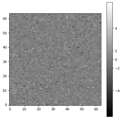
拉伸也可以与其他拉伸相结合,就像变换一样。结果 CompositeStretch 可用于像其他拉伸一样规格化Matplotlib图像。例如,复合拉伸可以拉伸负值的残余图像:
import numpy as np
import matplotlib.pyplot as plt
from astropy.visualization.stretch import SinhStretch, LinearStretch
from astropy.visualization import ImageNormalize

# Transforms normalized values [0,1] to [-1,1] before stretch and then back
stretch = LinearStretch(slope=0.5, intercept=0.5) + SinhStretch() + \
    LinearStretch(slope=2, intercept=-1)

# Image of random Gaussian noise
rng = np.random.default_rng()
image = rng.normal(size=(64, 64))
fig, ax = plt.subplots()
# ImageNormalize normalizes values to [0,1] before applying the stretch
norm = ImageNormalize(stretch=stretch, vmin=-5, vmax=5)
im = ax.imshow(image, origin='lower', norm=norm, cmap='gray')
fig.colorbar(im)
