20.4. 图像预处理的应用#
本部分介绍遥感中常用的图像预处理应用。 目标是从原始的、未经处理的产品(几何学和辐射测量学)生成可在地理信息系统中使用的图像。
20.4.1. 光学图像的辐射处理#
本节回顾了纠正多光谱卫星图像辐射测量的常用方法,主要受到Ose 等人的启发。 [ose16] 。
大气效应和许多其他机制会改变图像的辐射测量:地形效应、大气散射、方向效应(与太阳角、观测角或表面性质有关)。 本章中我们不提供可用的纠正方法。
传感器接收的光能量是与大气层和地球表面多次相互作用的结果。 在大气中,扩散和吸收机制减弱辐射。能量然后被地球表面吸收、传输和/或反射, 如 图 20.36 所示。
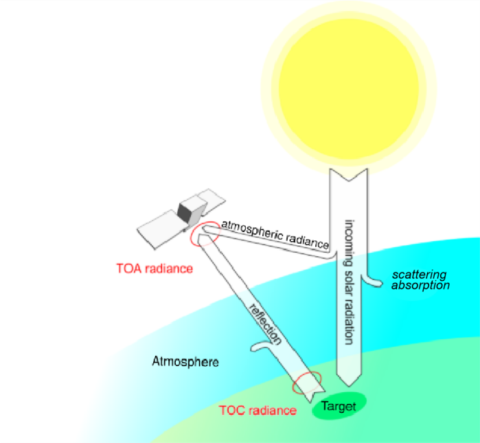
图 20.36 太阳辐射、大气和地球表面之间的相互作用#
反射能量、表面辐射或冠层顶部(TOC)辐射穿过大气层第二次;则传感器记录表观辐射或大气顶部(TOA)辐射。 在遥感中,将原始像素转换为TOA或TOC反射率(这是反射能量的一部分, 相对于射入能量)通常用于处理时间序列上的辐射指数分析:
原始像素到辐射度:传感器记录的数值之间的关系并且辐射度是每个通道的线性函数。这组函数的参数来源于传感器校准曲线, 并且通常在产品的元数据中可用。
辐射到TOA反射率:TOA反射率是反射到地球表面和大气层的传感器。 因此,它在[0,1]范围内具有连续值允许在两个或多个图像之间进行相对比较。 TOA反射率和TOA辐射率之间的关系是每个通道的线性函数。这些参数来自地球-太阳距离, 太阳光照和仰角。它们通常存在于产品的元数据中。
TOC反射率:TOC反射率取决于反射率和透射率气氛。因此,由于两个主要困难,计算很困难: 首先,大气条件不均匀。其次,它们并不总是在ROI内可用。计算TOC反射率有两种主要方法:
辐射传输建模(6S方法):该方法需要气象信息(压力、温度、湿度等),温度、不同气体的量、气溶胶的成分等), 光学特性(可视距离、透明度等),以及表面特性(均匀或非均匀反射率, 方向效应、土地利用类型等)加上用于计算辐射的参数;
使用不变目标进行校正:这组方法仅依赖于可用信息,以推断图像内部的大气特性。在最受欢迎的, 暗目标减影法基于辐射测量的目标不变量(例如山丘阴影)来计算校正参数。
在下面的练习中,我们使用 OpticalCalibration 应用程序计算Spot 6图像的反射率。
步骤说明#
浏览文件,浏览文件系统以到达要进行放射性修正的图像位置。
在Spot 6产品目录树中,图像的名称如下: “IMG_... TIF“(用于TIFF图像)或“IMG _... JP2”(用于jpeg2000图像)。 其元数据命名如下:“DIM _..”包含用于计算OTA反射率的参数的HTML。
图像和元数据文件必须在Dimap兼容性表格中具有名称:
“DIM _SPOT6 _ MS _..._1.XML”用与元数据文件。
“IMG _SPOT6 _MS _..._1_RxCy.TIF”用于图像。
如果文件的命名不同,OTB 函数可能无法正确访问metrix文件。 在这种情况下,用户必须指定所有参数(日期、角度、收益、偏差等)。
注:OTB 支持以下传感器的光学校准: QuickBird、Ikonos、WorldView(1、2和3)、Formosat、Spot 4/5/6/7、Pleiades。 对于这些传感器,所有参数都在产品的元数据中自动读取。
显示帮助#
执行 otbcli_OpticalCalibration (不带参数)以显示应用程序描述:
otbcli_OpticalCalibration
然后打印应用程序描述:
This is the OpticalCalibration application, version
5.2.1
Perform optical calibration TOA/TOC (Top Of
Atmosphere/Top Of Canopy). Supported sensors: QuickBird,
Ikonos, WorldView2, Formosat, Spot5, Pleiades, Spot6.

For other sensors the application also allows providing
calibration parameters manually.
Complete documentation: http://www.orfeo-toolbox.org/Applications/OpticalCalibration.html
Parameters:
 -progress <boolean>
Report progress
MISSING -in <string> Input
(mandatory)
MISSING -out <string> [pixel]
Output
[pixel=uint8/uint16/int16/uint32/int32/float/double]
(default value is float) (mandatory)
 -ram <int32>
Available RAM (Mb) (optional, off by default, default
value is 128)
 -level <string>
Calibration Level [toa/toatoim/toc] (mandatory, default
value is toa)
 -milli <boolean>
Convert to milli reflectance (optional, off by default)
 -clamp <boolean> Clamp
of reflectivity values between [0, 100] (optional, on
by default)
 -acqui.minute <int32>
Minute (mandatory, default value is 0)
 -acqui.hour <int32> Hour
(mandatory, default value is 12)
 -acqui.day <int32> Day
(mandatory, default value is 1)
 -acqui.month <int32> Month
(mandatory, default value is 1)
 -acqui.year <int32> Year
(mandatory, default value is 2000)
 -acqui.fluxnormcoeff <float> Flux
Normalization (optional, off by default)
 -acqui.sun.elev <float> Sun
elevation angle (°) (mandatory, default value is 90)
 -acqui.sun.azim <float> Sun
azimuth angle (°) (mandatory, default value is 0)
 -acqui.view.elev <float>
Viewing elevation angle (°) (mandatory, default value
is 90)
 -acqui.view.azim <float>

Viewing azimuth angle (°) (mandatory, default value is
0)
 -acqui.gainbias <string> Gains
| biases (optional, off by default)
 -acqui.solarilluminations <string> Solar
illuminations (optional, off by default)
 -atmo.aerosol <string>
Aerosol Model
[noaersol/continental/maritime/urban/desertic]
(mandatory, default value is noaersol)
 -atmo.oz <float> Ozone
Amount (optional, on by default, default value is 0)
 -atmo.wa <float> Water
Vapor Amount (optional, on by default, default value is
2.5)
 -atmo.pressure <float>
Atmospheric Pressure (optional, on by default, default
value is 1030)
 -atmo.opt <float>
Aerosol Optical Thickness (optional, on by default,
default value is 0.2)
 -atmo.aeronet <string>
Aeronet File (optional, off by default)
 -atmo.rsr <string>
Relative Spectral Response File (optional, off by
default)
 -atmo.radius <int32>
Window radius (adjacency effects) (optional, off by
default, default value is 2)
 -atmo.pixsize <float> Pixel
size (in km) (optional, on by default, default value is
1)
 -inxml <string> Load
otb application from xml file (optional, off by
default)
Examples:
otbcli_OpticalCalibration -in QB_1_ortho.tif -level toa
-out OpticalCalibration.tif
设置参数#
如果输入图像符合dimap格式,则自动设置“acqui”参数组。参数组“atmo”仅用于TOC反射率。
其他参数:
“级别”是指校正的类型(可能的值是“toa”、“toc”或“toatom”);
反射率的值是浮动十进制数,小于1。“milli”参数用于将该值乘以1000, 以便这些值可以用16位编码,从而节省了磁盘空间(浮点数的一半)。
在本练习中,仅设置以下参数:
“in”:输入图像的文件名“ROI_2_XS_Ortho_GSD2016”;
“level” 到 “toa”;
“out”: 输出TOA反射率图像的文件名。
执行运行算法。
分析在原始图像(TOA修正之前)和TOA反射率图像上计算NDVI。
比较植被上的两个值:在QGIS中打开两个输出图像并使用“值工具”(来自“查看”>“面板”)。 如果不可用,请使用插件管理器搜索并安装)。
SAR辐射测量处理#
合成口径雷达(SAR)是一种用于通过利用雷达的运动来模拟更大的天线以更高的分辨率来数字化图像的雷达。 描述了移动平台观察目标P三次但采集角度不同的采集原理,如 图 20.37 。 SAR处理结合了这些获取,允许您提高长度L的原始天线的分辨率,以获得长度M的等效合成天线, 该天线对应于方位角方向上的平台路径。回声目标P将位于射程维度中的距离h处。
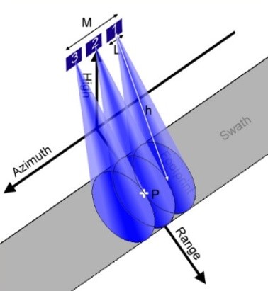
图 20.37 SAR采集原理#
SAR原理是一种主动微波遥感方法,允许用户白天或晚上捕获图像,在操作应用中具有明显的优势。 它被广泛用于从陆地到海洋应用的多种环境中。 例如,我们可以列出农业监测(通常与光学观察相结合)、洪水区检测、漏油(例如海上非法排放)或冰监测。
还有更先进的方法可以从SAR采集原理中派生出来;我们可以提到干涉测量法, 它使您能够生成数字地形图或测量小位移或旋光测量法,使您能够描述诸如植被类型等物体的特征。
移动平台上的雷达多次看到目标P(距离h),提供与长度M的合成天线相对应的分辨率(来源;维基百科)
SAR图像的辐射处理能够生成与反向散射信号直接相关的像素值。 事实上,反向散射信号的行为取决于表面特征,尤其是凹凸度、土壤湿度以及几何形状(偶极、角反射器)。
对于光学图像,辐射校准将数字转换为物理量。一般来说,1级地球观测产品不包括这些更正。 因此,应用这种校准来获取反向散射信号的物理值和表面属性非常重要。 它还允许您在来自潜在不同传感器的不同图像之间执行协调。
SAR校准主要包括计算以下量:
Beta Nought(:sup:“°”):或雷达亮度,对应于单位面积的反射率,以倾斜范围表示。
Sigma Nought(:sup:“°”):这对应于雷达反向散射系数,直接为与观察到的表面特性有关。 这代表了用平面假设考虑的像素。这个无单位值通常表示为单位为分贝(dB)。
Gamma_Nught(:sup:“°”):由入射角归一化的雷达后向散射系数。
为了计算这些操作,SAR图像产品通常提供元数据,允许您将像素值转换为这些物理量。
这些量可以使用OTB 应用程序 SARCalibration 计算。
该应用程序的文档可在CookBook [OTB 17 c]的“SAR处理”部分中找到。
支持 TerraSAR-X 、 Sentinel-1 和 Radarsat-2 传感器。
遥感图像的几何处理#
矫形矫正#
卫星图像的正射纠正包括将其呈现为在最低点(即垂直)处获取的图像。 此操作的目的是消除图像透视或磁贴和浮雕的影响, 如 图 20.38 、 图 20.39 所示, 正射矫正产生的图像能够测量距离、角度和表面。
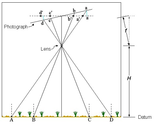
图 20.38 多光谱栅格传感器图像#
图“多光谱栅格传感器图像”倾斜位移是物体在倾斜照片上的图像位置与其在真正垂直照片上的理论位置的移动。 这是由于曝光时照片平面相对于基准平面倾斜的结果。 这种效果在上图中得到了证明。尽管A-B和C-D之间的距离在基准平面上相同, 但它们在照片平面上的相应表示则不同(即a带c-d之间的距离不相等)(来源:OSSSIM)。

图 20.39 正射矫正后的图像#
图“正射矫正后的图像”浮雕位移是物体在特定基准上方的高度引起的图像位置的移动。 对于垂直或近垂直摄影,移动从最低点呈放射状发生。这种效果如上图所示。 尽管A-B和C-D之间的距离在基准上相同平面,它们在照片平面上的相应表示不相同(即A-B和C-D之间的距离不相等)(来源:OSSSIM)
通常,封装非正射纠正产品的图像文件不具有地理参考元数据。 元数据通常在另一个文件中提供,专门用于封装。 例如,“Spot 6 Raster Sensor”图像的标题不包含任何地理参考信息; 所有与采集相关的元数据都包含在ML文档(dimap格式)中。 该图像无法直接在地理信息系统中使用,因为它没有附加坐标参考系。 只能以像素坐标显示,如 图 20.38 (a)。 正射矫正包括对图像应用几何变换。 经过正射纠正后,一个基准(测地系统)就会附加到图像上。 包含正射纠正图像(例如,GeoTivf)的文件就具有描述空间信息的元数据。 地理信息系统中常用的元数据包括:
空间参照系;
以空间参考系为单位的左上像素(图像原点)坐标;
以空间参考系为单位的X和Y维度的像素大小。
该空间信息可以计算每个像素的地图坐标。 这允许将正射纠正图像叠加到地图或任何其他正射纠正图像( 图 20.39 (b))。
为了对卫星图像进行正射纠正,通常使用以下信息:
图像和传感器模型;
DEM .
传感器模型描述了所有传感器采集参数,因此允许在地球表面上精确定位像素。 物理传感器模型源自轨道信息(获取时传感器的位置和方位), 但还有其他模型包括大气影响或接收站进行的处理(例如,在地图投影中对图像进行重新采样时)。 通常,模型的实施是特定于特定传感器的(例如,扫帚、推扫帚、针孔、帧摄像头、合成孔径雷达等)。 也有用数学近似(如多项式、几何级数等)表示的传感器模型,它们取代了模拟物理变换的方程(“替换模型”)。 另一类传感器模型包括提供图像的变换网格。 这些模型总是从采集的物理参数中得出,但它们的目标是提高执行速度而损害精度(变换是简单的内插, 而不是复杂的、严格的和非线性的建模)。 数字地形模型是适于由图像处理工具(即,通常是栅格)使用的陆地区域的地形的表示。 数字地形模型需要能够在三维空间中定位地球表面上的一个点,这是使用传感器模型所必需的。
在下面的练习中,我们对“Spot 6 Raster”传感器图像执行正射纠正(“ROI_3_P_Sensor_GSD2016”)。 将使用产品的传感器模型(如元数据中定义的)以及数字降雨模型。 接下来,OTB 应用程序将在命令线上被调用。
首先,我们使用 DownloadSRTMTiles 应用程序下载正射纠正图像所需的数字地形模型部分。
该应用程序确定原始图像及其相关传感器模型的坐标,以定位要下载的数字地形模型的相关部分。
步骤指令#
创建一个文件夹,在文件系统上创建一个“DEM _Tiles”目录。
此目录将用于托管 DownloadSRTMFiles 应用程序下载的数字高程模型文件。
在文件系统上创建“DEM _Tiles”目录。
此目录将用于托管将由 DownloadSRTMTiles 应用程序下载的数字海拔模型文件。
获取EM#
使用下载SRTMTiles应用程序检索数字地形模型的有用部分。 作为此应用程序的输入,将输入以下参数:
“il”:要检索数字模型的原始图像(“ROI_3_P_Sensor_GSD2016”);
“mode.download.outdir”:之前创建的目录“ DEM _Tiles”,我们想要在其中存储数字海拔模型的文件。
执行以下命令(将 < > 替换 DEM _Tiles 为包含数字海拔模型切片的目录的完整路径):
otbcli_DownloadSRTMTiles -mode.download.outdir << DEM _Tiles>> -il
rawInputImage.TIF
执行运行命令行。
该应用程序显示与图像覆盖的区域对应的下载文件的名称。
2017年3月22日14:05:37:Application.logger(Info)在USGSserver上找到瓦片,网址:http://dds.cr.usgs.gov/srtm/version2_1/SRTM3/Africa/N48W003.hgt.zip
2017年3月22日14:05:38:Application.logger(Info)在USGSserver上找到瓦片,网址:http://dds.cr.usgs.gov/srtm/version2_1/SRTM3/Africa/N48W004.hgt.zip
2017年3月22日14:05:39:Application.logger(Info)在USGSserver上找到瓦片,网址:http://dds.cr.usgs.gov/srtm/version2_1/SRTM3/Africa/N49W003.hgt.zip
2017年3月22日14:05:39:Application.logger(Info)在USGSserver上找到瓦片,网址:http://dds.cr.usgs.gov/srtm/version2_1/SRTM3/Africa/N49W004.hgt.zip
使用“DownloadSRMTTiles”应用程序下载SRTM数字海拔模型瓦片,然后,可以使用 Orthorectification 应用程序。
步骤指令#
显示应用程序描述执行
otbcli_Orthorectification ,没有参数来显示应用程序描述:
otbcli_OrthoRectification
然后打印应用程序描述:
This is the OrthoRectification application, version 5.2.1
This application allows ortho-rectification of optical images from
supported sensors.
Complete documentation: http://www.orfeotoolbox.org/Applications/OrthoRectification.html
Parameters:
-progress <boolean> Report progress
MISSING -io.in <string> Input
Image (mandatory)
MISSING -io.out <string> [pixel] Output
Image [pixel=uint8/uint16/int16/uint32/int32/float/double]
(default value is float) (mandatory)
-map <string> Output
Cartographic Map Projection
[utm/lambert2/lambert93/wgs/epsg] (mandatory, default value is utm)
-map.utm.zone <int32> Zone number (mandatory, default value is 31)
-map.utm.northhem <boolean> Northern Hemisphere (optional, off by
default)
-map.epsg.code <int32> EPSG Code
(mandatory, default value is 4326)
-outputs.mode <string>
Parameters estimation modes
[auto/autosize/autospacing/outputroi/orthofit] (mandatory, default value
is auto)
MISSING -outputs.ulx <float> Upper Left X (mandatory)
MISSING -outputs.uly <float> Upper Left Y (mandatory)
MISSING -outputs.sizex <int32> Size X (mandatory)
MISSING -outputs.sizey <int32> Size Y (mandatory)
MISSING -outputs.spacingx <float> Pixel Size X (mandatory)
MISSING -outputs.spacingy <float> Pixel Size Y (mandatory)
-outputs.lrx <float> Lower right X (optional, off by default)
-outputs.lry <float> Lower right Y (optional, off by default)
-outputs.ortho <string> Model ortho-image (optional, off by default)
-outputs.isotropic <boolean> Force isotropic spacing by default
(optional, on by default)
-outputs.default <float> Default pixel value (optional, on by default,
default value is 0)
-elev.dem <string>  DEM  directory (optional, off by default)
-elev.geoid <string> Geoid File (optional, off by default)
-elev.default <float> Default elevation (mandatory, default value is 0)
-interpolator <string>
Interpolation [bco/nn/linear] (mandatory, default value is bco)
-interpolator.bco.radius <int32> Radius for bicubic interpolation
(mandatory, default value is 2)
-opt.rpc <int32> RPC modeling (points per axis) (optional, off by
default, default value is 10)
-opt.ram <int32> Available
RAM (Mb) (optional, off by default, default value is 128)
-opt.gridspacing <float>
Resampling grid spacing (optional, on by default, default value is 4)
-inxml <string> Load otb application from xml file (optional, off by
default)
Examples: otbcli_OrthoRectification -io.in
QB_TOULOUSE_MUL_Extract_500_500.tif -io.out
QB_Toulouse_ortho.tif
设置参数设置以下参数:
“io.in”:输入图像文件名(即我们想要正射纠正的图像,“ROI_3_P_Sensor_GSD2016”), 后跟扩展文件名“?&skipcarto=true”。需要此扩展文件名来启用OrthoReady产品的正射纠正, 即:OrthoReady2A[]级的QuickBird、GeoEye、WV2和WV3[]产品,Spot-6/7光栅传感器。 这些产品具有伪坐标参考系这不能直接在地理信息系统中使用图像。 “&skipcarto=true”扩展文件名将忽略这些不需要的元数据。
“io.out”:输出图像的路径。由于Spot 6图像是在16个无符号比特上编码的,可以将像素类型设置为uint16。
“map”:选择用于法国大都市的地图投影“lambert93”。
“elev.dem”:“dem_Tiles”目录,包含数字高程模型图块。
参数的默认值适合当前可用的大多数图像。
然而,调整其中一些可能是有用的,以减少计算时间以进行快速预览:
“插值器”:如第5.3.1.2节所述,处理时间在很大程度上取决于插值器。最近邻插值器最快:选择“nn”以最小化计算时间。
“opt.gridspacing”:以地图单位确定变形网格的网格大小。该值越高,变形越粗糙,而且计算时间成本更低。 应该注意的是定义小于以下值的网格尺寸通常不是很有用图像像素的大小。 原则上,网眼尺寸为等于几个像素大小的变形网格就足够了:对于1.5m处的全色Spot 6图像, 对应于10个像素。当变形网格尺寸较小时数字地形模型和图像像素间距小,地形非常粗糙。
执行运行该过程(将 < > 替换 DEM _Tiles 为包含数字立面模型切片的目录的完整路径)。
otbcli_OrthoRectification
-io.in "PATH/TO/IMG_SPOT6_..._1_R1C1.TIF?&skipcarto=true"
-io.out roiOrtho.tif -map lambert93
-elev.dem << DEM _Tiles>> -interpolator nn
-opt.gridspacing 15
可视化将正射纠正图像导入QGIS并可视化。
评估DEM贡献#
在不指定数字地形模型的情况下再次运行应用程序: 这样,在正射纠正过程中仅使用轨道参数,而不使用任何海拔信息。
otbcli_OrthoRectification
-io.in "PATH/TO/IMG_SPOT6_..._1_R1C1.TIF?&skipcarto=true"
-io.out roiOrtho_no_dem.tif -map lambert93
-interpolator nn
-opt.gridspacing 15
将输出图像导入QGIS并可视化。
直观地比较使用和不使用数字海拔模型的正射纠正图像的平面测量。
“正矫正”申请
用地面控制点进行正射矫正#
最近的传感器模型通常能够以几米的相对误差实现图像参考。 然而,这种准确性并不总是可以接受的,尤其是当图像旨在进行小规模地理定位或变化检测时。 下一节介绍地面控制点的使用,这些点是用于改进传感器模型的参考点。 因此,图像以接近参考图像的准确度进行正射纠正。 本节介绍了实现这一目标的方法。
第一步包括提取不变点对。 因此,每个对由要进行正射纠正的图像上的第一不变点和参考图像上的第二点构成。
通过参考图像,可以手动识别点对。 但是,这种识别可以自动执行。 计算机视觉领域越来越多的算法使得检测和识别不同数字图像之间的相似元素变得更容易。 其中包括Sift[99]和SURF [BAY06] ,它们用于当前的许多应用, 如数字摄影中的场景自动创建,如 图 20.40 。
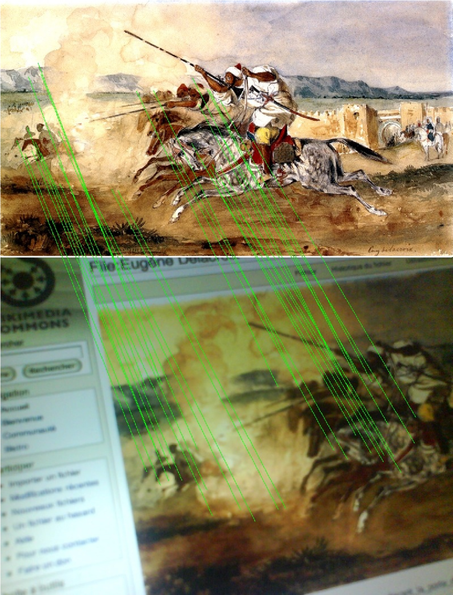
图 20.40 通过SIFT方法匹配两个图像的结果示例#
通过SIFT方法匹配两个图像的结果示例(Fantasia ou Jeu de la poudre,Devant la ported ' entée de la ville de Méquinez, 作者:Eugène Delacroix,1782年)(来源:维基百科)
SIFS和SURF都在OTB 应用程序中实现,名为“HomologousPointsDetection”。无论选择哪种算法(SFT或SURF),方法如下:
从图像中提取关键点:关键点具有尺度和旋转不变性。SIFT描述符是128个元素的向量,而SURF描述符是64个元素。
关键点匹配:基于描述符之间的欧几里德距离。目标是形成最接近的描述符对。 因此,两幅图像上的同源点根据它们的描述符进行匹配。
一旦获得多个同源点,可以稍微修改传感器模型的参数,以便更好地拟合参考点。 此步骤包括生成新的传感器模型这最小化了在前一步骤中提取的点对之间的二次误差。 OTB
RefineSensorModel应用程序执行此操作。最后一步包括使用新的改进传感器模型进行正射纠正。
在以下练习中,将使用额外控制点对Spot 6 RasterSenser(“ROI_3_P_Sensor_GSD2016”)图像进行正射纠正。 光学图像“ROI_3_P_Ortho_IGN 2015”将用作参考图像。 实施的步骤如下:
1)计算关键点(SIFS)来创建对,即地面控制点 HomologousPointExtraction 应用程序;
2)使用成对的地面控制点完善传感器模型 RefineSensorModel 应用程序;
3)使用精确的传感器模型进行正射矫正 Orthorection 应用)。
在以下示例中,应用程序将从命令行使用。 这种方法提供的一个有趣的可能性是创建脚本来链接上述三个步骤的能力。
为了减少每个步骤的处理时间,我们将仅处理输入的Spot 6 Raster Sensor图像的一个子集。
ExtractROI 应用程序用于提取图像的部分以及该区域特定的传感器模型。
传感器模型是由 ExtractROI 从"dimap"元数据中自动提取的,并将其作为输出图像,
扩展名为".geom"。
步骤指令#
提取投资回报率
使用 otbcli_ExtractROI 从"Spot 6 Raster Sensor"图像中提取任何"1000 x1000"像素的区域(无论起源如何)。
使用扩展名为“?&skipcarto=true”的输入图像的扩展文件名。
输入以下命令:
otbcli_ExtractROI -startx 200 -starty 200 -sizex 1000
-sizey 1000
-in "PATH/TO/IMG_SPOT6_..._1_R1C1.TIF?&skipcarto=true"
-out roi.tif
检查生成的文件使用文件资源管理器,确保已创建以下文件:
输出图像,采用GeoTIFF格式(.tif);
将与输出图像相关联的传感器模型存储在".geom"文件中。除扩展名外,此文件必须与输出图像同名。
ExtractROI 应用程序应该从"Dimap Spot 6"中提取传感器元数据,并将其合成在".geom"文件中。
后者可以通过简单的文本编辑器打开。
使用 ExtractROI 应用程序使用相关传感器模型提取图像区域
在此步骤中,我们提取了输入图像的子集,以及特定于该区域的传感器模型。
然而,此操作的主要目标是缩小图像的大小以加速过程。
如果希望在整个图像(而不仅仅是一个小区域)上继续此实践的步骤,则有必要提取特定于整个图像的传感器模型:
为此,请使用 ReadImage Info 应用程序。
该应用程序有两个强制参数,
即用于输入图像的“in”参数(输入图像)和用于存储传感器模型的“outkwl”参数(输出关键字列表)。
在进一步讨论之前,让我们对之前提取的子集图像进行正射纠正。
步骤指令#
进行正射矫正,使用 otbcli_Orthorectification 矫正使用上一节中描述的方法对子集图像执行正射矫正。
注意: 您不需要使用具有扩展名“?&”的扩展文件名skipcarto=true”,因为在使用ExtractROI应用程序提取区域时已经完成了这一操作。
otbcli_OrthoRectification -io.in roi.tif -io.out roiOrtho.tif -map
lambert93
-elev.dem << DEM _Tiles>> -interpolator nn
-opt.gridspacing 15
可视化将生成的图像导入QGIS
表5.19.使用 Orthorectification 应用程序对提取的图像进行正射矫正
下一步(如表5.20所示)包括使用OTB 应用程序同源点来提取点对。
步骤指令#
显示帮助
在没有参数的情况下执行 otbcli_Orthorectification 以显示应用程序描述:
otbcli_HomologousPointsExtraction
然后打印应用程序描述:
This is the HomologousPointsExtraction application, version 5.2.1

Compute homologous points between images using keypoints

Complete documentation: http://www.orfeo-toolbox.org/Applications/HomologousPointsExtraction.html

Parameters:

-progress <boolean> Report progress

MISSING -in1 <string> Input Image 1 (mandatory)

-band1 <int32> Input band 1 (mandatory, default value is 1)

MISSING -in2 <string> Input Image 2 (mandatory)

-band2 <int32> Input band 2 (mandatory, default value is 1)

-algorithm <string> Keypoints detection algorithm [surf/sift]
(mandatory, default value is surf)

-threshold <float> Distance threshold for matching (mandatory, default
value is 0.6)

-backmatching <boolean> Use backmatching to filter matches. (optional,
off by default)

-mode <string> Keypoints search mode [full/geobins] (mandatory, default
value is full)

-mode.geobins.binsize <int32> Size of bin (mandatory, default value is
256)

-mode.geobins.binsizey <int32> Size of bin (y direction) (optional, off
by default)

-mode.geobins.binstep <int32> Steps between bins (mandatory, default
value is 256)

-mode.geobins.binstepy <int32> Steps between bins (y direction)
(optional, off by default)

-mode.geobins.margin <int32> Margin from image border to start/end bins
(in pixels) (mandatory, default value is 10)

-precision <float> Estimated precision of the colocalisation function
(in pixels). (mandatory, default value is 0)

-mfilter <boolean> Filter points according to geographical or sensor
based colocalisation (optional, off by default)

-2wgs84 <boolean> If enabled, points from second image will be exported
in WGS84 (optional, off by default)

-elev.dem <string>  DEM  directory (optional, off by default)

-elev.geoid <string> Geoid

File (optional, off by default)

-elev.default <float>

Default elevation (mandatory, default value is 0)

MISSING -out <string> Output file with tie points (mandatory)

-outvector <string> Output vector file with tie points (optional, off by
default)

-inxml <string> Load otb application from xml file (optional, off by
default)

Examples:

otbcli_HomologousPointsExtraction -in1 sensor_stereo_left.tif in2
sensor_stereo_right.tif -mode full -out homologous.txt
该应用程序具有许多输入参数。
首先,有两个输入图像:
“in1”:图像1(我们想要几何校正的图像);
“in2”:图像2(参考图像“ROI_3_P_Ortho_IGN2015”)。
对于每张图像,一个额外的参数定义要使用的通道(分别为“band 1”和“band 2”)。 然后,参数“算法”允许您在两种算法之间进行选择,用于检测不变点(SIFS或SURF)。
无论选择的算法如何,以下参数都适用:
“阈值”:介于0和1之间的检测阈值。当接近1时,创建了大量的点对。当接近0时,创建了少量的点对。 点的关联是在描述符空间(SIFT或SURF)中完成的阈值应用于到最近描述符的距离与到第二最近描述符的距离;
“反向匹配”:当此布尔值为TRUE时,只有当该标准之前已经从图像1到图像2进行了验证,反之亦然。 这最大限度地减少了糟糕匹配的数量;
“模式”允许您在两种处理模式之间进行选择:
in “geobins” mode, images will be processes in subregions;
− “binsize”: size of subregions;
− “binstep”: step between two subregions;
− “margin”: margin around each subregion;
In “full” mode, images are processed entirely. We do not recommend processing full images because of the amount of memory it would require. In addition, keypoint pairing can be a very long operation when there are a big number of points.
“precision”:当“mfilter”为true时,此值为最大值图像1的点和图像2的点之间的距离(以物理单位表示)。
当一对点之间的距离大于该值时,拒绝一对点;
“2wgs84”:为真时,坐标以WGS84导出;
“out”是包含点的输出表格文件的文件名。
“outvector”是输出向量层的文件名。它是可选的,但有助于直观地比较已生成的地面控制点。
设置参数#
提取相应的点。 这些点将保存在.CSV格式的表格文件中,并保存在".shp"文件(ESRI Shapefile格式)中。
使用SIFT算法;
使用“geobin”模式,保留其默认子参数;
当距离大于30米时,拒绝成对的点(将“精度”设置为30,将“mfilter”设置为1);
别忘了在elev.dem中设置数字高程模型。
执行运行命令行:
otbcli_HomologousPointsExtraction -in1 roi_sensor.tif -in2
PATH\TO\ROI_3_P_Ortho_IGN2015\IMG_S6P_2015032636879163CP_R1C 1.tif
-2wgs84 1 -mfilter 1 -precision 25 -mode geobins -out points.txt
-outvector deplacement_points.shp -elev.dem << DEM _DIR>> -backmatching 1
分析将参考图像导入QGIS。
导入正射矫正后图像的子集。
最后,打开之前生成的矢量图层并分析两张图像之间的位移。 可以修改渲染风格(颜色、宽度)以更好地可视化矢量图层中的点。
表5.20.使用 HomologousPointsExtraction 应用程序提取同名点
我们现在可以继续进行步骤(2)。
在这一步中,使用前一步中生成的控制点来细化传感器模型。
RefineSensorModel 应用程序生成一个新的传感器模型,可以最大限度地减少平方误差。
步骤指令#
显示帮助
在没有参数的情况下执行 otbcli_Orthorectification 以显示帮助:
otbcli_RefineSensorModel
然后打印应用程序描述:
This is the RefineSensorModel application, version 5.2.1

Perform least-square fit of a sensor model to a set of tie points

Complete documentation: http://www.orfeotoolbox.org/Applications/RefineSensorModel.html

Parameters:

-progress <boolean> Report progress

MISSING -ingeom <string> Input geom file (mandatory)

MISSING -outgeom <string> Output geom file (mandatory)

MISSING -inpoints <string> Input file containing tie points (mandatory)

-outstat <string> Output file containing output precision statistics
(optional, off by default)

-outvector <string> Output vector file with residues (optional, off by
default)

-map <string> Output

Cartographic Map Projection [utm/lambert2/lambert93/wgs/epsg]
(mandatory, default value is utm)

-map.utm.zone <int32> Zone number (mandatory, default value is 31)

-map.utm.northhem <boolean> Northern Hemisphere (optional, off by
default)

-map.epsg.code <int32> EPSG Code (mandatory, default value is 4326)

-elev.dem <string>  DEM  directory (optional, off by default)

-elev.geoid <string> Geoid File

(optional, off by default)

-elev.default <float> Default elevation (mandatory, default value is 0)

-inxml <string> Load otb

application from xml file (optional, off by default)

Examples:

otbcli_RefineSensorModel -ingeom input.geom -outgeom output.geom
-inpoints points.txt -map epsg -map.epsg.code 32631
设置参数#
设置以下输入参数:
“ingeom”:对传感器模型(.geom)进行细化;
“输入点”:包含地面控制点的文件(生成输出文件“out”通过同源点提取);
“outgeom”:应用程序将创建的新传感器模型的文件名(.geom);
“outstations”:导出点精度统计数据的文件(表)。通常,对于每个地面控制点,偏移(以物理单位表示)、误差、高程等。
执行运行命令行:
otbcli_RefineSensorModel -ingeom roi_sensor.geom -outgeom
roi_sensor_refined.geom -outstat refine_stats.csv -outvector
residus_deplacement_points.shp -map lambert93 -elev.dem
<< DEM _DIR>> -inpoints points.txt
分析在电子表格软件中打开“outstat”输出文件,如 图 20.41 ,分析地面控制点的位置误差。
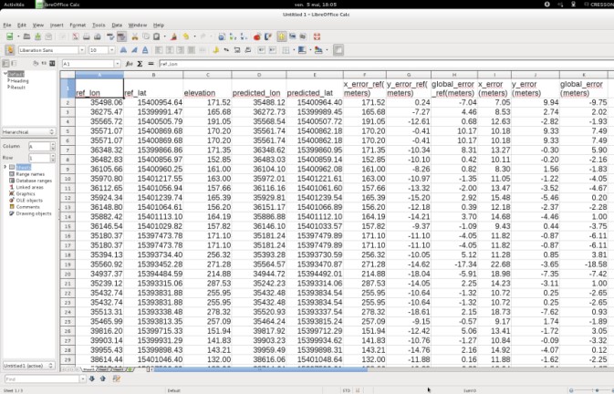
图 20.41 统计表#
将统计数据与QGIS中的是两次层进行比较。
还可以在地面控制点文件(用于“inpoints”参数)中手动删除具有较大全局误差(即错误)的点, 然后再次运行细化传感器过程。
表5.21.使用 RefineSensorModel 应用程序完善传感器模型
表5.22中描述的步骤包括执行第5.3.2.3.1节中解释的正射矫正, 但使用新的传感器模型而不是原始的传感器模型。
步骤指令#
设置参数
在控制台中,输入与第5.3.2.3.1节所述相同的参数。
按照下面的说明完成命令行。
设置输入图像
设置输入图像参数,并将新传感器型号设置为使用扩展文件名,如下所示:
otbcli_OrthoRectification
-io.in "roi.tif?&refined_sensor.geom" -io.out roiOrtho.tif
-map lambert93 -elev.dem << DEM _Tiles>> -interpolator nn
-opt.gridspacing 15
其中:
roi.tif是输入图像子集;
refined_sensor.geom是
RefineSensorModel应用程序生成的新的精炼传感器模型。
执行运行命令行。
分析在QGIS中打开输出图像,使用参考图像将物理定位的精度与其他生产图像进行比较:
无DEM的正射纠正;
使用DEM进行正射纠正。
表5.22.使用“正射矫正”应用程序,通过精细传感器模型进行正射矫正
全色锐化#
对地观测卫星通常具有一个全彩色传感器和一系列空间分辨率较低的多光谱传感器。 为了利用这两种信息来源,人们开发了多种技术来产生多光谱图像,该图像具有与全彩色图像相同的空间分辨率。 这种技术被称为锐化。
在本节中,我们将介绍在OTB 中实现的两种全景细化方法: 相对分量替换(RC)和Bayesian Data Fusion(BDF)。
RCS方法,如 图 20.42 :合并图像的一种简单方法是考虑在分辨率相同的情况下,全色图像是多光谱图像通道的总和。 一旦图像以相同的分辨率重新采样,就可以进行融合:其想法是对全色通道图像应用低通滤波器, 使其光谱内容(在傅里叶域中)接近多光谱图像。然后,多光谱图像被滤波后的全色图像归一化,并与原始全色图像相乘。 该方法的唯一参数是低通滤波器半径。
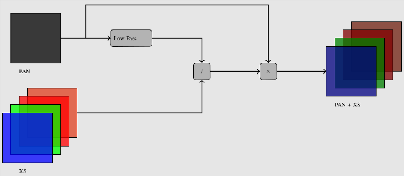
图 20.42 RCS Panelishering方法#
BDF方法基于频谱带和全彩色通道之间的统计关系。最好处理感兴趣的区域,而不是整个图像。 我们不会深入探讨该方法的技术细节;但感兴趣的读者可以获得原始出版物[FAS 08]。 该方法的一个有趣特征是可以相对于频谱信息对空间信息进行加权,从而可以根据需要调整其使用。 例如,照片解释更加关注图像的清晰度:这可以通过赋予全彩色通道中包含的信息更大的权重来实现。 请注意,在他们的文章中,作者提出了一组适应城市、林业、农业和地中海环境的参数值。
在下面的练习中,
叠加 和 全景锐化 应用程序与Spot 6图像(“ROI_1_Bundle_Ortho_GSD2015”)的多光谱通道(XS图像)和多色通道(SPAN图像)一起使用。
ReadImage Info 应用程序用于检查图像属性,例如像素间隔和光谱带数量。
步骤指令#
获取图像信息,在XS图像上使用ReadImage Info应用程序来获取图像属性:
otbcli_ReadImageInfo -in IMG _SPOT6_MS_..._1_R1C1.TIF
该信息由应用程序显示,如 图 20.43 。 请注意图像的大小(行数、列数)、像素间距(以地图单位)和XS图像中的通道数量。
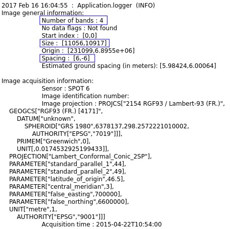
图 20.43 条带数量、大小和间距(蓝色)#
有关此图的彩色版本,请参阅www.iste.co.uk/baghdadi/qgis1.zip
对PAN图像重复该操作。
比较图像的大小和分辨率(PAN图像的分辨率必须是XS图像的四倍,XS图像的分辨率只有一个通道与四倍)。
提取ROI为了加快全景清晰操作,我们将仅处理输入图像的一个子集。
使用ExtractROI应用程序提取此PAN图像子集:
otbcli_ExtractROI -in IMG_SPOT6_P_..._1_R1C1.TIF
-sizex 1000 -sizey 1000 -out pan_roi.tif
重新采样XS图像
在此步骤中,我们以与先前创建的PANimage ROI相同的范围和像素间距对XS图像进行重新采样。
无论采用哪种方法,这一步都是全景化的先决条件
选择了事实上,XS图像的内插不包括在 Panshiring 应用程序中,因为它是一个独立的过程。
选择半径为两个像素的双三次字形
在四倍大的PAN图像上插值XS图像以避免伪影(请参阅第5.3.2.3.1节)。
选择以下参数:
“参考输入”:设置PAN图像ROI的路径(在初步步骤中提取);
“要重新投影的图像”:设置要重新采样的XS图像的路径;
“插值”:选择半径为两个像素的“双三次”。
将其他参数保留为默认值。图像已经进行正射纠正,无需输入大地水准面或数字海拔模型。
重新分配并执行在PAN图像上重新分配XS图像:
otbcli_Superimpose -inm IMG _SPOT6_MS_..._1_R1C1.TIF -inr pan_roi.tif
-out ms_roi_resamp.tif
执行RCS,使用 Panshiring 命令行应用程序。指定图像的路径:
XS图像:设置上一步在PAN图像ROI上重采样的XS图像的文件名;
PAN图像:设置PAN图像ROI的文件名。
将“方法”参数设置为“rcs”,指定输出图像的文件名并执行算法。
otbcli_Pansharpening -inp pan_roi.tif
-inxs ms_roi_resamp.tif -out pansharp_rcs.tif -method rcs
执行重复上一步,但将参数“方法”更改为“Bayes”:
BDS
otbcli_Pansharpening -inp pan_roi.tif
-inxs ms_roi_resamp.tif -out pansharp_bds.tif -method bayes
分析将PAN和XS图像导入QGIS。
从RCS和BDS方法导入图像并进行视觉比较。
表5.23.使用“Pansheling”应用程序进行光学图像的Pansheling
图像镶嵌#
与要覆盖的广阔区域相比,遥感器的足迹通常很小:
因此,需要生成卫星图像镶嵌来将大量小足迹场景组合到单个镶嵌中。
Mosaic 应用程序满足了这一需求。可选的矢量数据可用于选择输入图像边界。
与大多数涉及图像重采样的 OTB 应用程序一样,插值方法可以出现(双三次、线性或最近邻居)。
另一方面,土地利用、表面照明、大气条件和传感器引入的邻近图像之间存在颜色差异。 该应用程序包括一种颜色协调方法,可以最大限度地减少图像重叠部分中的像素差异, 如 图 20.44 、如 图 20.45 。 这种差异可以在图像的原始辐射色彩空间中或在适合自然场景中人类视觉的去相关色彩空间中计算 [CRE15] 。
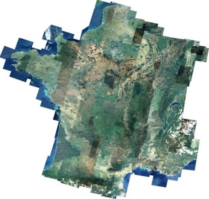
图 20.44 自然色镶嵌#
图 20.45 自然彩色镶嵌#
图 a)自然色镶嵌,没有协调(132 RapidEye场景,5 m空间分辨率); b)具有协调的自然彩色镶嵌。
有关此图的彩色版本,请参阅 www.iste.co.uk/baghdadi/qgis1.zip
在下面的练习中,我们从3个SPOT 6图像(“ROI_2_XS_Ortho_GSD2016”、“ROI_3_XS_Ortho_GSD2015”和“ROI_4_XS_ Ortho_GSD2017”)生成输出镶嵌图案。
步骤指令#
显示帮助,不带参数地执行otbSYS_Mosaic以显示帮助:
otbcli_Mosaic
然后打印应用程序描述:
This is the Mosaic application, version 5.2.1 Perform mosaicking of
input images

Complete documentation: http://www.orfeotoolbox.org/Applications/Mosaic.html

Parameters:

-progress <boolean>

Report progress

MISSING -il <string list> Input Images (mandatory)

-vdcut <string list> Input VectorDatas for composition (optional, off by
default)

-vdstats <string list> Input

VectorDatas for statistics (optional, off by default)

-comp.feather <string> Feathering method [none/large/slim] (mandatory,
default value is none)

-comp.feather.slim.exponent <float> Transition smoothness (Unitary
exponent = linear transition) (optional, on by default, default value is
1)

-comp.feather.slim.lenght <float> Transition length (In cartographic
units) (optional, off by default)

-harmo.method <string> harmonization method [none/band/rgb] (mandatory,
default value is none)

-harmo.cost <string> harmonization cost function [rmse/musig/mu]
(mandatory, default value is rmse)

MISSING -out <string> [pixel]

Output image

[pixel=uint8/uint16/int16/uint32/int32/float/double] (default value is
float) (mandatory)

-interpolator <string>

Interpolation [nn/bco/linear] (optional, off by default,

default value is nn)

-interpolator.bco.radius <int32> Radius for bicubic interpolation
(mandatory, default value is 2)

-output.spacing <float> Pixel

Size (optional, off by default)

-tmpdir <string> Directory where to write temporary files (optional, off
by default)

-distancemap.sr <float> Distance map images sampling ratio (mandatory,
default value is 10)

-ram <int32> Available RAM (Mb) (optional, off by default, default value
is 128)

-inxml <string> Load otb application from xml file (optional, off by
default)
创建镶嵌,使用“-il”参数选择输入图像。
保留其他默认参数,输入输出文件名,并验证命令行:
otbcli_Mosaic-il PATH/TO/ROI_2…/IMG_SPOT6_..._1_R1C1.TIF
/PATH/TO/ROI_3…/IMG_SPOT6_..._1_R1C1.TIF
/PATH/TO/ROI_4…/IMG_SPOT6_..._1_R1C1.TIF -out mosaic.tif
将生成的镶嵌图片导入QGIS并可视化。
创建自然色彩和谐的镶嵌
使用“-il”参数选择输入图像。
将参数“-harmo.method”设置为“rgb”以协调镶嵌非自然色彩。 保留其他默认设置,输入输出图像的文件名,并验证命令行:
otbcli_Mosaic-il PATH/TO/ROI_2…/IMG_SPOT6_..._1_R1C1.TIF
/PATH/TO/ROI_3…/IMG_SPOT6_..._1_R1C1.TIF
/PATH/TO/ROI_4…/IMG_SPOT6_..._1_R1C1.TIF
-harmo.method rgb -out mosaic_harmo_rgb.tif
将生成的镶嵌图片导入QGIS并可视化。与之前生成的镶嵌进行比较。
表5.24.使用“Mosaic”应用程序镶嵌图像
20.4.2. 参考文献#
OSE K., DEMAGISTRI L., CORPETTI T.,“Multispectral SatelliteImage Processing”, in BAGHDADI N., ZRIBI M. (eds), Optical RemoteSensing of Land Surface: Techniques and Methods, ISTE Press, London andElsevier, Oxford, 2016.
BAY H., TUYTELAARS T., VAN GOOL L., “SURF: Speeded Up RobustFeatures”, in LEONARDIS A., BISCHOF H., PINZ A. (eds), Computer Vision– ECCV 2006, Springer, Berlin, 2006.