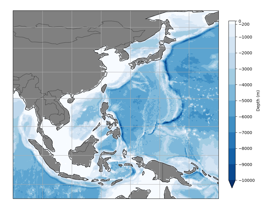
海洋测深学

制作海洋海底深度地图，展示 cartopy.io.shapereader.Reader 接口.该数据是从Natural Earth获得的一系列10 m分辨率的嵌套多边形，源自NASA SRTM Plus产品。由于数据集包含一个zipfile，其中有多个代表不同深度的ShapFile，因此该示例演示了使用通用Shape Reader界面而不是专用界面手动下载和读取它们 cartopy.feature.NaturalEarthFeature 接口.

from glob import glob

import matplotlib
import matplotlib.pyplot as plt
import numpy as np

import cartopy.crs as ccrs
import cartopy.feature as cfeature
import cartopy.io.shapereader as shpreader


def load_bathymetry(zip_file_url):
    """Read zip file from Natural Earth containing bathymetry shapefiles"""
    # Download and extract shapefiles
    import io
    import zipfile

    import requests
    r = requests.get(zip_file_url)
    z = zipfile.ZipFile(io.BytesIO(r.content))
    z.extractall("ne_10m_bathymetry_all/")

    # Read shapefiles, sorted by depth
    shp_dict = {}
    files = glob('ne_10m_bathymetry_all/*.shp')
    assert len(files) > 0
    files.sort()
    depths = []
    for f in files:
        depth = '-' + f.split('_')[-1].split('.')[0]  # depth from file name
        depths.append(depth)
        bbox = (90, -15, 160, 60)  # (x0, y0, x1, y1)
        nei = shpreader.Reader(f, bbox=bbox)
        shp_dict[depth] = nei
    depths = np.array(depths)[::-1]  # sort from surface to bottom
    return depths, shp_dict


if __name__ == "__main__":
    # Load data (14.8 MB file)
    depths_str, shp_dict = load_bathymetry(
        'https://naturalearth.s3.amazonaws.com/' +
        '10m_physical/ne_10m_bathymetry_all.zip')

    # Construct a discrete colormap with colors corresponding to each depth
    depths = depths_str.astype(int)
    N = len(depths)
    nudge = 0.01  # shift bin edge slightly to include data
    boundaries = [min(depths)] + sorted(depths+nudge)  # low to high
    norm = matplotlib.colors.BoundaryNorm(boundaries, N)
    blues_cm = matplotlib.colormaps['Blues_r'].resampled(N)
    colors_depths = blues_cm(norm(depths))

    # Set up plot
    subplot_kw = {'projection': ccrs.LambertCylindrical()}
    fig, ax = plt.subplots(subplot_kw=subplot_kw, figsize=(9, 7))
    ax.set_extent([90, 160, -15, 60], crs=ccrs.PlateCarree())  # x0, x1, y0, y1

    # Iterate and plot feature for each depth level
    for i, depth_str in enumerate(depths_str):
        ax.add_geometries(shp_dict[depth_str].geometries(),
                          crs=ccrs.PlateCarree(),
                          color=colors_depths[i])

    # Add standard features
    ax.add_feature(cfeature.LAND, color='grey')
    ax.coastlines(lw=1, resolution='110m')
    ax.gridlines(draw_labels=False)
    ax.set_position([0.03, 0.05, 0.8, 0.9])

    # Add custom colorbar
    axi = fig.add_axes([0.85, 0.1, 0.025, 0.8])
    ax.add_feature(cfeature.BORDERS, linestyle=':')
    sm = plt.cm.ScalarMappable(cmap=blues_cm, norm=norm)
    fig.colorbar(mappable=sm,
                 cax=axi,
                 spacing='proportional',
                 extend='min',
                 ticks=depths,
                 label='Depth (m)')

    # Convert vector bathymetries to raster (saves a lot of disk space)
    # while leaving labels as vectors
    ax.set_rasterized(True)