

创建一个新的坐标类(用于人马座流)#
本文档详细描述了如何对自定义球坐标系进行子分类和定义,如中所讨论的 定义新框架 以及文档字符串 BaseCoordinateFrame .在本例中,我们将定义由射手座矮星系(以下称为SGR;如Mazenski等人2003年所定义)的轨道平面定义的坐标系。Sgr坐标系通常用两个角坐标来指代, \(\Lambda,B\) .
为此,我们需要定义 BaseCoordinateFrame 它知道每个支持的表示中的坐标系角度的名称和单位。在这种情况下,我们支持 SphericalRepresentation 带有“Lambda”和“Beta”。然后我们必须定义从这个坐标系到其他内置系统的转换。这里我们将使用银河系坐标,由 Galactic 课
参见
- 的 gala package
定义恒星流坐标系的多个天体坐标系。
- Majenski等人2003
“人马座矮星系的两微米全天空巡天视图。I.人马座核心和潮汐臂的形态”,https://arxiv.org/abs/astro-ph/0304198
- Law & Mazenski 2010
“射手座矮星系:三轴银河光环中的进化模型”,https://arxiv.org/abs/1003.1132
- David Law的SGR信息页面
>>> import matplotlib.pyplot as plt
>>> import numpy as np
>>> import astropy.coordinates as coord
>>> from astropy import units as u
>>> from astropy.coordinates import frame_transform_graph
>>> from astropy.coordinates.matrix_utilities import matrix_transpose, rotation_matrix
第一步是创建一个新类,我们将其称为 Sagittarius 并使其成为 BaseCoordinateFrame :
>>> class Sagittarius(coord.BaseCoordinateFrame):
...     """A Heliocentric spherical coordinate system defined by the orbit
...     of the Sagittarius dwarf galaxy, as described in
...         https://ui.adsabs.harvard.edu/abs/2003ApJ...599.1082M
...     and further explained in
...         https://www.stsci.edu/~dlaw/Sgr/.
...
...     Parameters
...     ----------
...     representation : `~astropy.coordinates.BaseRepresentation` or None
...         A representation object or None to have no data (or use the other keywords)
...     Lambda : `~astropy.coordinates.Angle`, optional, must be keyword
...         The longitude-like angle corresponding to Sagittarius' orbit.
...     Beta : `~astropy.coordinates.Angle`, optional, must be keyword
...         The latitude-like angle corresponding to Sagittarius' orbit.
...     distance : `~astropy.units.Quantity`, optional, must be keyword
...         The Distance for this object along the line-of-sight.
...     pm_Lambda_cosBeta : `~astropy.units.Quantity`, optional, must be keyword
...         The proper motion along the stream in ``Lambda`` (including the
...         ``cos(Beta)`` factor) for this object (``pm_Beta`` must also be given).
...     pm_Beta : `~astropy.units.Quantity`, optional, must be keyword
...         The proper motion in Declination for this object (``pm_ra_cosdec`` must
...         also be given).
...     radial_velocity : `~astropy.units.Quantity`, optional, keyword-only
...         The radial velocity of this object.
...     """
...     default_representation = coord.SphericalRepresentation
...     default_differential = coord.SphericalCosLatDifferential
...     frame_specific_representation_info = {
...         coord.SphericalRepresentation: [
...             coord.RepresentationMapping("lon", "Lambda"),
...             coord.RepresentationMapping("lat", "Beta"),
...             coord.RepresentationMapping("distance", "distance"),
...         ]
...     }
将其逐行分解,我们将类定义为 BaseCoordinateFrame .然后我们包括一个描述性文档字符串。最后一行是类级属性,指定数据的默认表示、速度信息的默认差异,以及从表示对象使用的属性名称到要由 Sagittarius frame.在这种情况下,我们覆盖球形表示中的名称,但不对旋转体或圆柱体等其他表示进行任何操作。
接下来,我们必须定义从这个坐标系到其他内置坐标系的转换;我们将使用银河系坐标。我们可以通过定义返回变换矩阵的函数来做到这一点,或者简单地定义接受坐标并返回新系统中新坐标的函数来做到这一点。由于到射手座坐标干的变换只是银河系坐标的球形旋转,因此我们将定义一个返回此矩阵的函数。我们将首先使用预定的欧拉角和 rotation_matrix 辅助功能:
>>> SGR_PHI = (180 + 3.75) * u.degree  # Euler angles (from Law & Majewski 2010)
>>> SGR_THETA = (90 - 13.46) * u.degree
>>> SGR_PSI = (180 + 14.111534) * u.degree
使用x约定生成旋转矩阵(请参阅Goldstein):
>>> SGR_MATRIX = (
...     np.diag([1.0, 1.0, -1.0])
...     @ rotation_matrix(SGR_PSI, "z")
...     @ rotation_matrix(SGR_THETA, "x")
...     @ rotation_matrix(SGR_PHI, "z")
... )
由于我们已经构造了上面的变换(旋转)矩阵,而旋转矩阵的逆就是它的转置,因此所需的变换函数非常简单:
>>> @frame_transform_graph.transform(
...     coord.StaticMatrixTransform, coord.Galactic, Sagittarius
... )
... def galactic_to_sgr():
...     """Compute the Galactic spherical to heliocentric Sgr transformation matrix."""
...     return SGR_MATRIX
装饰器 @frame_transform_graph.transform(coord.StaticMatrixTransform, coord.Galactic, Sagittarius) 将此函数注册到 frame_transform_graph 作为坐标变换。在函数内部,我们返回之前定义的旋转矩阵。
然后我们通过使用旋转矩阵的转置来注册逆变换(计算速度比逆变换更快):
>>> @frame_transform_graph.transform(
...     coord.StaticMatrixTransform, Sagittarius, coord.Galactic
... )
... def sgr_to_galactic():
...     """Compute the heliocentric Sgr to spherical Galactic transformation matrix."""
...     return matrix_transpose(SGR_MATRIX)
现在我们已经记录了之间的这些转变 Sagittarius 和 Galactic ,我们可以在 any 坐标系和 Sagittarius (as只要对方系统有转型的路径 Galactic ).例如,从ICRS坐标转换为 Sagittarius ,我们会做:
>>> icrs = coord.SkyCoord(280.161732 * u.degree, 11.91934 * u.degree, frame="icrs")
>>> sgr = icrs.transform_to(Sagittarius)
>>> print(sgr)
<SkyCoord (Sagittarius): (Lambda, Beta) in deg
    (346.81830652, -39.28360407)>
或者,从 Sagittarius 框架到ICRS坐标(在这种情况下,是沿着 Sagittarius x-y平面):
>>> sgr = coord.SkyCoord(
...     Lambda=np.linspace(0, 2 * np.pi, 128) * u.radian,
...     Beta=np.zeros(128) * u.radian,
...     frame="sagittarius",
... )
>>> icrs = sgr.transform_to(coord.ICRS)
>>> print(icrs)
<SkyCoord (ICRS): (ra, dec) in deg
    [(284.03876751, -29.00408353), (287.24685769, -29.44848352),
     (290.48068369, -29.81535572), (293.7357366 , -30.1029631 ),
     ...]>
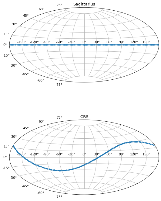
例如,我们现在将绘制两个坐标系中的点:
>>> fig, axes = plt.subplots(2, 1, figsize=(8, 10), subplot_kw={"projection": "aitoff"})
>>> axes[0].set_title("Sagittarius")
>>> axes[0].plot(
...     sgr.Lambda.wrap_at(180 * u.deg).radian,
...     sgr.Beta.radian,
...     linestyle="none",
...     marker=".",
... )
>>> axes[0].grid(visible=True)
>>> axes[1].set_title("ICRS")
>>> axes[1].plot(
...     icrs.ra.wrap_at(180 * u.deg).radian, icrs.dec.radian, linestyle="none", marker="."
... )
>>> axes[1].grid(visible=True)
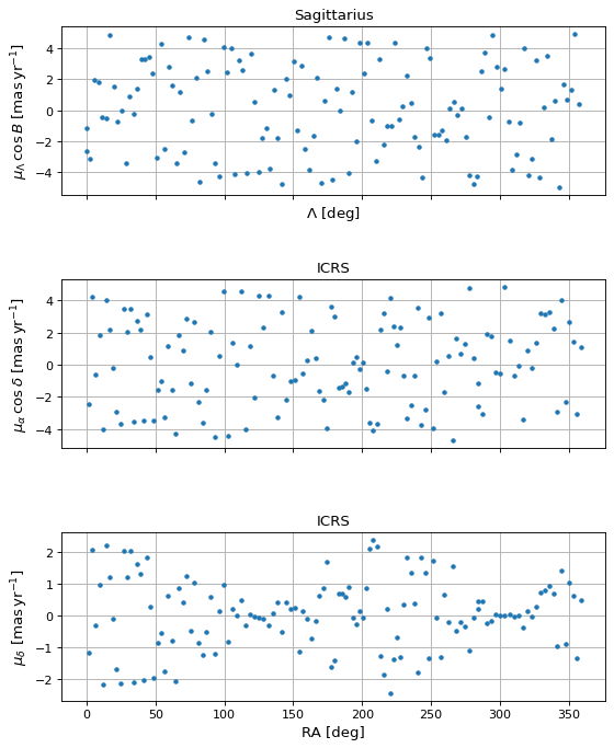
这个特定的变换只是一个球形旋转,这是不带载体偏差的仿射变换的特殊情况。因此,速度分量的转换也受到本地支持:
>>> sgr = coord.SkyCoord(
...     Lambda=np.linspace(0, 2 * np.pi, 128) * u.radian,
...     Beta=np.zeros(128) * u.radian,
...     pm_Lambda_cosBeta=np.random.uniform(-5, 5, 128) * (u.mas / u.yr),
...     pm_Beta=np.zeros(128) * (u.mas / u.yr),
...     frame="sagittarius",
... )
>>> icrs = sgr.transform_to(coord.ICRS)
>>> print(icrs)
<SkyCoord (ICRS): (ra, dec) in deg
    [(284.03876751, -29.00408353), (287.24685769, -29.44848352),
     ...,
     ...]>
>>> fig, axes = plt.subplots(3, 1, figsize=(8, 10), sharex=True)
>>> axes[0].set_title("Sagittarius")
>>> axes[0].plot(
...     sgr.Lambda.degree, sgr.pm_Lambda_cosBeta.value, linestyle="none", marker="."
... )
>>> axes[0].set_xlabel(r"$\Lambda$ [deg]")
>>> axes[0].set_ylabel(
...     rf"$\mu_\Lambda \, \cos B$ [{sgr.pm_Lambda_cosBeta.unit.to_string('latex_inline')}]"
... )
>>> axes[0].grid(visible=True)
>>> axes[1].set_title("ICRS")
>>> axes[1].plot(icrs.ra.degree, icrs.pm_ra_cosdec.value, linestyle="none", marker=".")
>>> axes[1].set_ylabel(
...     rf"$\mu_\alpha \, \cos\delta$ [{icrs.pm_ra_cosdec.unit.to_string('latex_inline')}]"
... )
>>> axes[1].grid(visible=True)
>>> axes[2].set_title("ICRS")
>>> axes[2].plot(icrs.ra.degree, icrs.pm_dec.value, linestyle="none", marker=".")
>>> axes[2].set_xlabel("RA [deg]")
>>> axes[2].set_ylabel(rf"$\mu_\delta$ [{icrs.pm_dec.unit.to_string('latex_inline')}]")
>>> axes[2].grid(visible=True)
>>> plt.draw()
