插值 (scipy.interpolate )

目录

• 插值 (scipy.interpolate )

  • 一维插值 (interp1d )

  • 多变量数据插值 (griddata )

  • 样条插值

    • 一维中的样条插值：程序化(interpolate.plXXX)

    • 一维中的样条插值：面向对象 (UnivariateSpline )

    • 二维样条线表示：程序化 (bisplrep )

    • 二维样条线表示：面向对象 (BivariateSpline )

  • 使用径向基函数进行平滑/插值

    • 一维示例

    • 二维示例

对于1维、2维和更高维的数据，SciPy中提供了几种常规插值工具：

• 表示插值的类 (interp1d )，给出了几种插值方法。

• 便利函数 griddata 提供N维(N=1，2，3，4，.)内插的简单接口。底层例程的面向对象接口也可用。

• 基于FORTRAN库FITPACK的一维和二维(平滑)三次样条插值函数。它们都是FITPACK库的过程接口和面向对象接口。

• 使用径向基函数的插值。

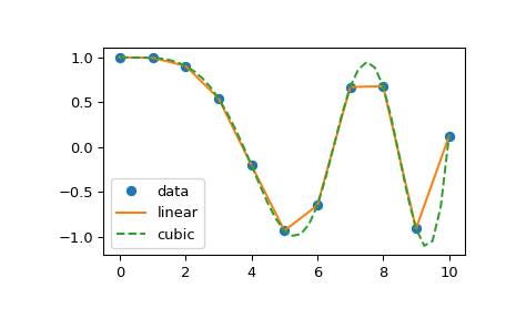
一维插值 (interp1d )

这个 interp1d 中的类 scipy.interpolate 是一种基于固定数据点创建函数的便捷方法，可以使用线性插值在给定数据定义的域内的任何位置计算该函数。通过传递组成数据的一维向量来创建此类的实例。此类的实例定义了一个 __call__ 方法，因此可以将其视为在已知数据值之间进行插值以获得未知值的函数(它还具有用于帮助的文档字符串)。边界处的行为可以在实例化时指定。下面的示例演示了它在线性样条插值和三次样条插值中的用法：

>>> from scipy.interpolate import interp1d

>>> x = np.linspace(0, 10, num=11, endpoint=True)
>>> y = np.cos(-x**2/9.0)
>>> f = interp1d(x, y)
>>> f2 = interp1d(x, y, kind='cubic')

>>> xnew = np.linspace(0, 10, num=41, endpoint=True)
>>> import matplotlib.pyplot as plt
>>> plt.plot(x, y, 'o', xnew, f(xnew), '-', xnew, f2(xnew), '--')
>>> plt.legend(['data', 'linear', 'cubic'], loc='best')
>>> plt.show()

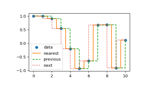
中的另一组插值 interp1d 是 nearest ， previous ，以及 next ，其中它们返回沿x轴最近的点、上一个点或下一个点。最近的和次要的可以被认为是因果插值过滤的特例。下面的示例使用与上一个示例中相同的数据演示它们的用法：

>>> from scipy.interpolate import interp1d

>>> x = np.linspace(0, 10, num=11, endpoint=True)
>>> y = np.cos(-x**2/9.0)
>>> f1 = interp1d(x, y, kind='nearest')
>>> f2 = interp1d(x, y, kind='previous')
>>> f3 = interp1d(x, y, kind='next')

>>> xnew = np.linspace(0, 10, num=1001, endpoint=True)
>>> import matplotlib.pyplot as plt
>>> plt.plot(x, y, 'o')
>>> plt.plot(xnew, f1(xnew), '-', xnew, f2(xnew), '--', xnew, f3(xnew), ':')
>>> plt.legend(['data', 'nearest', 'previous', 'next'], loc='best')
>>> plt.show()

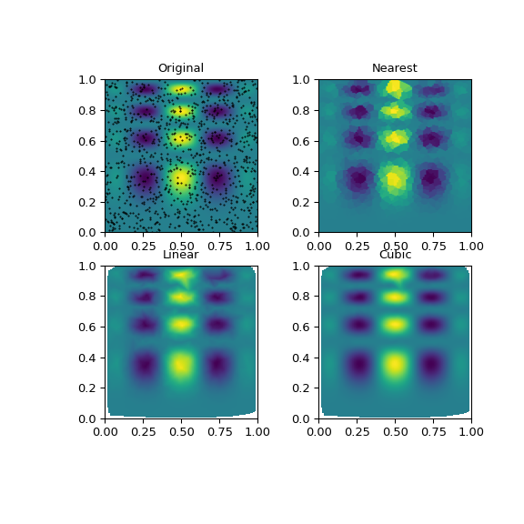
多变量数据插值 (griddata )

例如，假设您具有基础函数的多维数据 F(x，y) 你只知道点上的值 [(X[i]，y[i])] 它们不会形成规则的网格。

假设我们要对二维函数进行插值

>>> def func(x, y):
...     return x*(1-x)*np.cos(4*np.pi*x) * np.sin(4*np.pi*y**2)**2

在中的栅格上 [0, 1] X [0, 1]

>>> grid_x, grid_y = np.mgrid[0:1:100j, 0:1:200j]

但我们只知道它在1000个数据点的值：

>>> rng = np.random.default_rng()
>>> points = rng.random((1000, 2))
>>> values = func(points[:,0], points[:,1])

这可以通过以下方式完成 griddata --下面我们将尝试所有的插值方法：

>>> from scipy.interpolate import griddata
>>> grid_z0 = griddata(points, values, (grid_x, grid_y), method='nearest')
>>> grid_z1 = griddata(points, values, (grid_x, grid_y), method='linear')
>>> grid_z2 = griddata(points, values, (grid_x, grid_y), method='cubic')

可以看到，所有方法都在一定程度上重现了准确的结果，但对于此光滑函数，分段三次插值提供了最好的结果：

>>> import matplotlib.pyplot as plt
>>> plt.subplot(221)
>>> plt.imshow(func(grid_x, grid_y).T, extent=(0,1,0,1), origin='lower')
>>> plt.plot(points[:,0], points[:,1], 'k.', ms=1)
>>> plt.title('Original')
>>> plt.subplot(222)
>>> plt.imshow(grid_z0.T, extent=(0,1,0,1), origin='lower')
>>> plt.title('Nearest')
>>> plt.subplot(223)
>>> plt.imshow(grid_z1.T, extent=(0,1,0,1), origin='lower')
>>> plt.title('Linear')
>>> plt.subplot(224)
>>> plt.imshow(grid_z2.T, extent=(0,1,0,1), origin='lower')
>>> plt.title('Cubic')
>>> plt.gcf().set_size_inches(6, 6)
>>> plt.show()

样条插值

一维中的样条插值：程序化(interpolate.plXXX)

样条插值需要两个基本步骤：(1)计算曲线的样条表示，(2)在所需的点处计算样条。为了找到样条表示，有两种不同的方式来表示曲线并获得(平滑)样条系数：直接和参数化。直接法使用函数求出二维平面中曲线的样条表示 splrep 。前两个参数是唯一需要的参数，它们提供了 \(x\) 和 \(y\) 曲线的组成部分。正常输出是3元组， \(\left(t,c,k\right)\) ，包含结点， \(t\) ，这些系数 \(c\) 以及命令 \(k\) 样条线的。默认样条曲线顺序为三次，但可以使用INPUT关键字进行更改。 k.

对于N-D空间中的曲线，函数 splprep 允许以参数方式定义曲线。对于此函数，只需要1个输入参数。此输入是以下内容的列表 \(N\) -在N-D空间中表示曲线的数组。每个数组的长度是曲线点的数量，每个数组提供N维数据点的一个分量。参数变量与关键字自变量一起给出， u, ，它缺省为两个序列之间的等间距单调序列 \(0\) 和 \(1\) 。默认输出由两个对象组成：3元组， \(\left(t,c,k\right)\) ，包含样条表示和参数变量 \(u.\)

The keyword argument, s , is used to specify the amount of smoothing to perform during the spline fit. The default value of \(s\) is \(s=m-\sqrt{2m}\) where \(m\) is the number of data-points being fit. Therefore, if no smoothing is desired a value of \(\mathbf{s}=0\) should be passed to the routines.

一旦确定了数据的样条表示，就可以使用函数来计算样条 (splev )及其衍生物 (splev ， spalde )和任意两点之间的样条积分( splint )。此外，对于三次样条( \(k=3\) )对于8个或更多的结点，可以估计样条的根( sproot )。下面的示例演示了这些函数。

>>> import numpy as np
>>> import matplotlib.pyplot as plt
>>> from scipy import interpolate

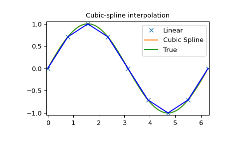
三次样条

>>> x = np.arange(0, 2*np.pi+np.pi/4, 2*np.pi/8)
>>> y = np.sin(x)
>>> tck = interpolate.splrep(x, y, s=0)
>>> xnew = np.arange(0, 2*np.pi, np.pi/50)
>>> ynew = interpolate.splev(xnew, tck, der=0)

>>> plt.figure()
>>> plt.plot(x, y, 'x', xnew, ynew, xnew, np.sin(xnew), x, y, 'b')
>>> plt.legend(['Linear', 'Cubic Spline', 'True'])
>>> plt.axis([-0.05, 6.33, -1.05, 1.05])
>>> plt.title('Cubic-spline interpolation')
>>> plt.show()

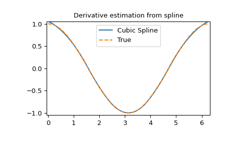
样条的导数

>>> yder = interpolate.splev(xnew, tck, der=1)
>>> plt.figure()
>>> plt.plot(xnew, yder, xnew, np.cos(xnew),'--')
>>> plt.legend(['Cubic Spline', 'True'])
>>> plt.axis([-0.05, 6.33, -1.05, 1.05])
>>> plt.title('Derivative estimation from spline')
>>> plt.show()

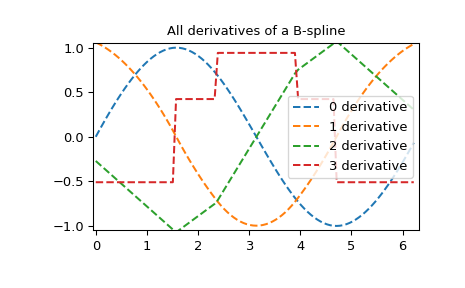
样条的所有导数

>>> yders = interpolate.spalde(xnew, tck)
>>> plt.figure()
>>> for i in range(len(yders[0])):
...    plt.plot(xnew, [d[i] for d in yders], '--', label=f"{i} derivative")
>>> plt.legend()
>>> plt.axis([-0.05, 6.33, -1.05, 1.05])
>>> plt.title('All derivatives of a B-spline')
>>> plt.show()

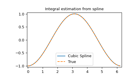
样条积分

>>> def integ(x, tck, constant=-1):
...     x = np.atleast_1d(x)
...     out = np.zeros(x.shape, dtype=x.dtype)
...     for n in range(len(out)):
...         out[n] = interpolate.splint(0, x[n], tck)
...     out += constant
...     return out

>>> yint = integ(xnew, tck)
>>> plt.figure()
>>> plt.plot(xnew, yint, xnew, -np.cos(xnew), '--')
>>> plt.legend(['Cubic Spline', 'True'])
>>> plt.axis([-0.05, 6.33, -1.05, 1.05])
>>> plt.title('Integral estimation from spline')
>>> plt.show()

样条的根

>>> interpolate.sproot(tck)
array([3.1416])

请注意， sproot 在近似区间的边缘找不到明显的解， \(x = 0\) 。如果我们在稍微大一点的间隔上定义样条，我们可以恢复两个根 \(x = 0\) 和 \(x = 2\pi\) ：

>>> x = np.linspace(-np.pi/4, 2.*np.pi + np.pi/4, 21)
>>> y = np.sin(x)
>>> tck = interpolate.splrep(x, y, s=0)
>>> interpolate.sproot(tck)
array([0., 3.1416])

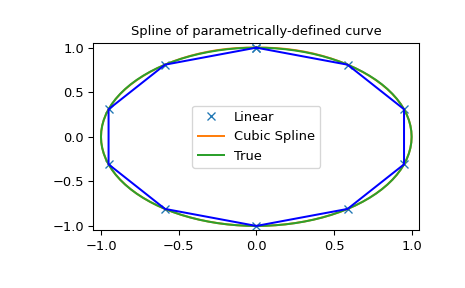
参数样条

>>> t = np.arange(0, 1.1, .1)
>>> x = np.sin(2*np.pi*t)
>>> y = np.cos(2*np.pi*t)
>>> tck, u = interpolate.splprep([x, y], s=0)
>>> unew = np.arange(0, 1.01, 0.01)
>>> out = interpolate.splev(unew, tck)
>>> plt.figure()
>>> plt.plot(x, y, 'x', out[0], out[1], np.sin(2*np.pi*unew), np.cos(2*np.pi*unew), x, y, 'b')
>>> plt.legend(['Linear', 'Cubic Spline', 'True'])
>>> plt.axis([-1.05, 1.05, -1.05, 1.05])
>>> plt.title('Spline of parametrically-defined curve')
>>> plt.show()

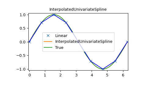
一维中的样条插值：面向对象 (UnivariateSpline )

还可以通过面向对象的界面使用上述样条曲线拟合功能。一维样条线是 UnivariateSpline class, and are created with the \(x\) and \(y\) components of the curve provided as arguments to the constructor. The class defines _ _CALL__，允许使用x轴值调用对象，样条线应在x轴值进行求值，并返回插值的y值。下面的子类示例中显示了这一点 InterpolatedUnivariateSpline 。这个 integral ， derivatives ，以及 roots 上也提供了方法 UnivariateSpline 对象，允许计算样条曲线的定积分、导数和根。

UnivariateSpline类还可用于通过提供非零值的平滑参数来平滑数据 s ，其含义与 s 的关键字 splrep 功能如上所述。这会导致样条线的节点少于数据点的数量，因此不再是严格意义上的插值样条线，而是平滑样条线。如果这不是所需的，则 InterpolatedUnivariateSpline 课程可用。它是的子类 UnivariateSpline 始终通过所有点(相当于将平滑参数强制设置为0)。下面的示例演示了这个类。

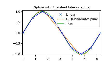
这个 LSQUnivariateSpline 类是的另一个子类 UnivariateSpline 。它允许用户使用参数显式指定内部结的数量和位置 t 。这允许创建具有非线性间距的自定义样条线，以便在某些域中进行插值，在其他域中进行平滑，或者更改样条线的特性。

>>> import numpy as np
>>> import matplotlib.pyplot as plt
>>> from scipy import interpolate

InterpolatedUnivariateSpline

>>> x = np.arange(0, 2*np.pi+np.pi/4, 2*np.pi/8)
>>> y = np.sin(x)
>>> s = interpolate.InterpolatedUnivariateSpline(x, y)
>>> xnew = np.arange(0, 2*np.pi, np.pi/50)
>>> ynew = s(xnew)

>>> plt.figure()
>>> plt.plot(x, y, 'x', xnew, ynew, xnew, np.sin(xnew), x, y, 'b')
>>> plt.legend(['Linear', 'InterpolatedUnivariateSpline', 'True'])
>>> plt.axis([-0.05, 6.33, -1.05, 1.05])
>>> plt.title('InterpolatedUnivariateSpline')
>>> plt.show()

具有非均匀结点的LSQUnivarateSpline

>>> t = [np.pi/2-.1, np.pi/2+.1, 3*np.pi/2-.1, 3*np.pi/2+.1]
>>> s = interpolate.LSQUnivariateSpline(x, y, t, k=2)
>>> ynew = s(xnew)

>>> plt.figure()
>>> plt.plot(x, y, 'x', xnew, ynew, xnew, np.sin(xnew), x, y, 'b')
>>> plt.legend(['Linear', 'LSQUnivariateSpline', 'True'])
>>> plt.axis([-0.05, 6.33, -1.05, 1.05])
>>> plt.title('Spline with Specified Interior Knots')
>>> plt.show()

二维样条线表示：程序化 (bisplrep )

对于2-D曲面的(平滑)样条拟合，函数 bisplrep 是有空的。此函数根据需要接受 1-D 阵列 x ， y ，以及 z ，表示曲面上的点 \(z=f\left(x,y\right).\) 默认输出为列表 \(\left[tx,ty,c,kx,ky\right]\) 其条目分别表示节点位置的分量、样条的系数和样条在每个坐标中的阶数。将该列表保存在单个对象中是方便的， tck, 以便可以轻松地将其传递给函数 bisplev 。关键字， s 可用于在确定适当的样条曲线时更改对数据执行的平滑量。默认值为 \(s=m-\sqrt{{2m}}\) ，在哪里 \(m\) 中的数据点的数量。 x，y， 和 z 矢量。因此，如果不需要平滑，则 \(s=0\) 应传递给 bisplrep 。

要计算二维样条线及其偏导数(直到样条线的阶数)，函数 bisplev 是必需的。此函数以前两个参数为参数 two 1-D arrays 其叉积指定了对样条线求值的域。第三个参数是 tck 从返回的列表 bisplrep 。如果需要，第四个和第五个参数提供 \(x\) 和 \(y\) 方向。

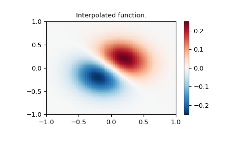
重要的是要注意，不应使用二维插值来查找图像的样条表示。所使用的算法不适用于大量输入点。信号处理工具箱包含更合适的算法，用于查找图像的样条表示。2-D插值命令用于插值2-D函数，如下例所示。此示例使用 mgrid NumPy中的命令，该命令对于在多个维度中定义“网格”非常有用。(另请参阅 ogrid 如果不需要全网格，则使用命令)。输出参数的数量和每个参数的维数由传入的索引对象的数量决定 mgrid 。

>>> import numpy as np
>>> from scipy import interpolate
>>> import matplotlib.pyplot as plt

在稀疏的20x20网格上定义函数

>>> x_edges, y_edges = np.mgrid[-1:1:21j, -1:1:21j]
>>> x = x_edges[:-1, :-1] + np.diff(x_edges[:2, 0])[0] / 2.
>>> y = y_edges[:-1, :-1] + np.diff(y_edges[0, :2])[0] / 2.
>>> z = (x+y) * np.exp(-6.0*(x*x+y*y))

>>> plt.figure()
>>> lims = dict(cmap='RdBu_r', vmin=-0.25, vmax=0.25)
>>> plt.pcolormesh(x_edges, y_edges, z, shading='flat', **lims)
>>> plt.colorbar()
>>> plt.title("Sparsely sampled function.")
>>> plt.show()

新的70x70网格上的插值函数

>>> xnew_edges, ynew_edges = np.mgrid[-1:1:71j, -1:1:71j]
>>> xnew = xnew_edges[:-1, :-1] + np.diff(xnew_edges[:2, 0])[0] / 2.
>>> ynew = ynew_edges[:-1, :-1] + np.diff(ynew_edges[0, :2])[0] / 2.
>>> tck = interpolate.bisplrep(x, y, z, s=0)
>>> znew = interpolate.bisplev(xnew[:,0], ynew[0,:], tck)

>>> plt.figure()
>>> plt.pcolormesh(xnew_edges, ynew_edges, znew, shading='flat', **lims)
>>> plt.colorbar()
>>> plt.title("Interpolated function.")
>>> plt.show()

二维样条线表示：面向对象 (BivariateSpline )

这个 BivariateSpline 类是 UnivariateSpline 班级。它及其子类以面向对象的方式实现上述FITPACK函数，允许实例化对象，通过将两个坐标作为两个参数传入，可以调用这些对象来计算样条值。

使用径向基函数进行平滑/插值

径向基函数可用于平滑/内插N维的散乱数据，但在进行观测数据范围之外的外推时应谨慎使用。

一维示例

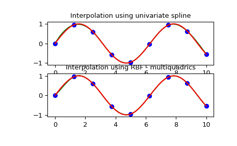
此示例比较 Rbf 和 UnivariateSpline 来自scipy.interpolate模块的类。

>>> import numpy as np
>>> from scipy.interpolate import Rbf, InterpolatedUnivariateSpline
>>> import matplotlib.pyplot as plt

>>> # setup data
>>> x = np.linspace(0, 10, 9)
>>> y = np.sin(x)
>>> xi = np.linspace(0, 10, 101)

>>> # use fitpack2 method
>>> ius = InterpolatedUnivariateSpline(x, y)
>>> yi = ius(xi)

>>> plt.subplot(2, 1, 1)
>>> plt.plot(x, y, 'bo')
>>> plt.plot(xi, yi, 'g')
>>> plt.plot(xi, np.sin(xi), 'r')
>>> plt.title('Interpolation using univariate spline')

>>> # use RBF method
>>> rbf = Rbf(x, y)
>>> fi = rbf(xi)

>>> plt.subplot(2, 1, 2)
>>> plt.plot(x, y, 'bo')
>>> plt.plot(xi, fi, 'g')
>>> plt.plot(xi, np.sin(xi), 'r')
>>> plt.title('Interpolation using RBF - multiquadrics')
>>> plt.show()

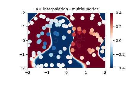
二维示例

此示例说明如何插值分散的二维数据：

>>> import numpy as np
>>> from scipy.interpolate import Rbf
>>> import matplotlib.pyplot as plt
>>> from matplotlib import cm

>>> # 2-d tests - setup scattered data
>>> rng = np.random.default_rng()
>>> x = rng.random(100)*4.0-2.0
>>> y = rng.random(100)*4.0-2.0
>>> z = x*np.exp(-x**2-y**2)
>>> edges = np.linspace(-2.0, 2.0, 101)
>>> centers = edges[:-1] + np.diff(edges[:2])[0] / 2.
>>> XI, YI = np.meshgrid(centers, centers)

>>> # use RBF
>>> rbf = Rbf(x, y, z, epsilon=2)
>>> ZI = rbf(XI, YI)

>>> # plot the result
>>> plt.subplot(1, 1, 1)
>>> X_edges, Y_edges = np.meshgrid(edges, edges)
>>> lims = dict(cmap='RdBu_r', vmin=-0.4, vmax=0.4)
>>> plt.pcolormesh(X_edges, Y_edges, ZI, shading='flat', **lims)
>>> plt.scatter(x, y, 100, z, edgecolor='w', lw=0.1, **lims)
>>> plt.title('RBF interpolation - multiquadrics')
>>> plt.xlim(-2, 2)
>>> plt.ylim(-2, 2)
>>> plt.colorbar()

上一页

优化 (scipy.optimize )

下一页

傅立叶变换 (scipy.fft )