空间数据结构和算法 (scipy.spatial )
scipy.spatial can compute triangulations, Voronoi diagrams, and convex hulls of a set of points, by leveraging the Qhull 类库。
此外,它还包含 KDTree 最近邻点查询的实现,以及各种度量中距离计算的实用程序。
Delaunay三角测量
Delaunay三角剖分是将一组点细分为一组不重叠的三角形,这样任何三角形的外接圆内都没有点。在实践中,这样的三角剖分往往会避免带有小角度的三角形。
可以使用以下方法计算Delaunay三角剖分 scipy.spatial 具体如下:
>>> from scipy.spatial import Delaunay
>>> points = np.array([[0, 0], [0, 1.1], [1, 0], [1, 1]])
>>> tri = Delaunay(points)
我们可以把它形象化:
>>> import matplotlib.pyplot as plt
>>> plt.triplot(points[:,0], points[:,1], tri.simplices)
>>> plt.plot(points[:,0], points[:,1], 'o')
并添加一些进一步的装饰:
>>> for j, p in enumerate(points):
...     plt.text(p[0]-0.03, p[1]+0.03, j, ha='right') # label the points
>>> for j, s in enumerate(tri.simplices):
...     p = points[s].mean(axis=0)
...     plt.text(p[0], p[1], '#%d' % j, ha='center') # label triangles
>>> plt.xlim(-0.5, 1.5); plt.ylim(-0.5, 1.5)
>>> plt.show()
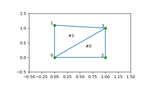
三角剖分的结构按以下方式编码: simplices 属性包含 points 组成三角形的数组。例如:
>>> i = 1
>>> tri.simplices[i,:]
array([3, 1, 0], dtype=int32)
>>> points[tri.simplices[i,:]]
array([[ 1. ,  1. ],
       [ 0. ,  1.1],
       [ 0. ,  0. ]])
此外,还可以找到相邻三角形:
>>> tri.neighbors[i]
array([-1,  0, -1], dtype=int32)
这告诉我们这个三角形有#0号三角形作为邻居,但没有其他邻居。此外,它还告诉我们邻居0与三角形的顶点1相对:
>>> points[tri.simplices[i, 1]]
array([ 0. ,  1.1])
事实上,从数字上,我们可以看到情况是这样的。
Qhull还可以对高维点集执行细分以简化(例如,在3-D中细分为四面体)。
共面点
重要的是要注意到,不是 all 由于形成三角剖分的数值精度问题,点必然显示为三角剖分的顶点。请考虑具有重复点的上述内容:
>>> points = np.array([[0, 0], [0, 1], [1, 0], [1, 1], [1, 1]])
>>> tri = Delaunay(points)
>>> np.unique(tri.simplices.ravel())
array([0, 1, 2, 3], dtype=int32)
请注意,重复的点#4不会作为三角剖分的顶点出现。这件事已被记录在案:
>>> tri.coplanar
array([[4, 0, 3]], dtype=int32)
这意味着点4位于三角形0和顶点3附近,但不包括在三角剖分中。
请注意,这种退化不仅可能是因为重复的点,也可能是由于更复杂的几何原因,即使在乍看起来表现良好的点集中也是如此。
但是,Qhull具有“qj”选项,该选项指示它随机扰乱输入数据,直到解决退化问题:
>>> tri = Delaunay(points, qhull_options="QJ Pp")
>>> points[tri.simplices]
array([[[1, 0],
        [1, 1],
        [0, 0]],
       [[1, 1],
        [1, 1],
        [1, 0]],
       [[1, 1],
        [0, 1],
        [0, 0]],
       [[0, 1],
        [1, 1],
        [1, 1]]])
出现了两个新的三角形。然而,我们看到它们是退化的,面积为零。
凸壳
凸包是包含给定点集中所有点的最小凸对象。
这些值可以通过中的qhull包装器进行计算。 scipy.spatial 具体如下:
>>> from scipy.spatial import ConvexHull
>>> rng = np.random.default_rng()
>>> points = rng.random((30, 2))   # 30 random points in 2-D
>>> hull = ConvexHull(points)
凸包被表示为一组N个1-D简化,在2-D中表示线段。存储方案与上面讨论的Delaunay三角剖分中的简化完全相同。
我们可以举例说明上述结果:
>>> import matplotlib.pyplot as plt
>>> plt.plot(points[:,0], points[:,1], 'o')
>>> for simplex in hull.simplices:
...     plt.plot(points[simplex,0], points[simplex,1], 'k-')
>>> plt.show()
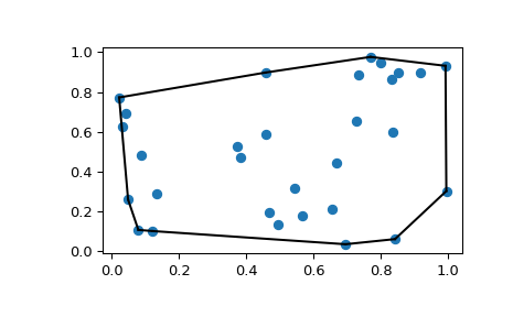
同样的情况也可以通过以下方式实现 scipy.spatial.convex_hull_plot_2d 。
Voronoi图
Voronoi图是将空间细分为一组给定点的最近邻域。
使用以下两种方法可以接近此对象 scipy.spatial 。首先,可以使用 KDTree 要回答“哪个点最接近这个点”的问题,并这样定义区域:
>>> from scipy.spatial import KDTree
>>> points = np.array([[0, 0], [0, 1], [0, 2], [1, 0], [1, 1], [1, 2],
...                    [2, 0], [2, 1], [2, 2]])
>>> tree = KDTree(points)
>>> tree.query([0.1, 0.1])
(0.14142135623730953, 0)
所以重点是 (0.1, 0.1) 属于区域 0 。在颜色方面:
>>> x = np.linspace(-0.5, 2.5, 31)
>>> y = np.linspace(-0.5, 2.5, 33)
>>> xx, yy = np.meshgrid(x, y)
>>> xy = np.c_[xx.ravel(), yy.ravel()]
>>> import matplotlib.pyplot as plt
>>> dx_half, dy_half = np.diff(x[:2])[0] / 2., np.diff(y[:2])[0] / 2.
>>> x_edges = np.concatenate((x - dx_half, [x[-1] + dx_half]))
>>> y_edges = np.concatenate((y - dy_half, [y[-1] + dy_half]))
>>> plt.pcolormesh(x_edges, y_edges, tree.query(xy)[1].reshape(33, 31), shading='flat')
>>> plt.plot(points[:,0], points[:,1], 'ko')
>>> plt.show()
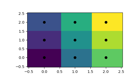
然而,这并没有给出作为几何对象的Voronoi图。
线和点的表示可以通过中的qhull包装器再次获得 scipy.spatial :
>>> from scipy.spatial import Voronoi
>>> vor = Voronoi(points)
>>> vor.vertices
array([[0.5, 0.5],
       [0.5, 1.5],
       [1.5, 0.5],
       [1.5, 1.5]])
Voronoi顶点表示形成Voronoi区域的多边形边的点集。在本例中,有9个不同的区域:
>>> vor.regions
[[], [-1, 0], [-1, 1], [1, -1, 0], [3, -1, 2], [-1, 3], [-1, 2], [0, 1, 3, 2], [2, -1, 0], [3, -1, 1]]
负值 -1 再次表示无穷远处的一个点。事实上,只有一个地区, [0, 1, 3, 2] ,是有界的。请注意,由于与上面的Delaunay三角剖分中类似的数值精度问题,Voronoi区域可能比输入点少。
将分隔区域的脊(二维中的线)描述为与凸面壳片类似的简化集合:
>>> vor.ridge_vertices
[[-1, 0], [-1, 0], [-1, 1], [-1, 1], [0, 1], [-1, 3], [-1, 2], [2, 3], [-1, 3], [-1, 2], [1, 3], [0, 2]]
这些数字表示组成线段的Voronoi顶点的索引。 -1 又是一个无穷远的点-12条直线中只有4条是有界线段,而其他的延伸到无穷远。
Voronoi山脊垂直于输入点之间绘制的线。还记录了每个脊对应的两个点:
>>> vor.ridge_points
array([[0, 3],
       [0, 1],
       [2, 5],
       [2, 1],
       [1, 4],
       [7, 8],
       [7, 6],
       [7, 4],
       [8, 5],
       [6, 3],
       [4, 5],
       [4, 3]], dtype=int32)
这些信息加在一起,足以构成完整的图表。
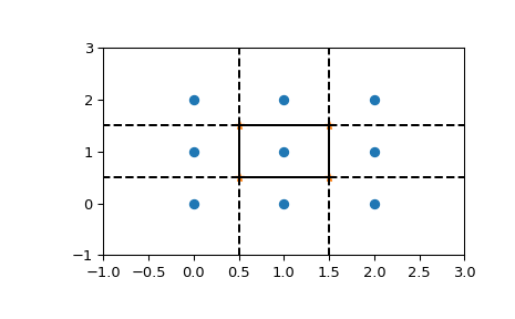
我们可以把它画成如下图。首先,点和Voronoi顶点:
>>> plt.plot(points[:, 0], points[:, 1], 'o')
>>> plt.plot(vor.vertices[:, 0], vor.vertices[:, 1], '*')
>>> plt.xlim(-1, 3); plt.ylim(-1, 3)
绘制有限线段与绘制凸壳一样,但现在我们必须注意无限边:
>>> for simplex in vor.ridge_vertices:
...     simplex = np.asarray(simplex)
...     if np.all(simplex >= 0):
...         plt.plot(vor.vertices[simplex, 0], vor.vertices[simplex, 1], 'k-')
延伸到无穷远的山脊需要稍微小心一点:
>>> center = points.mean(axis=0)
>>> for pointidx, simplex in zip(vor.ridge_points, vor.ridge_vertices):
...     simplex = np.asarray(simplex)
...     if np.any(simplex < 0):
...         i = simplex[simplex >= 0][0] # finite end Voronoi vertex
...         t = points[pointidx[1]] - points[pointidx[0]]  # tangent
...         t = t / np.linalg.norm(t)
...         n = np.array([-t[1], t[0]]) # normal
...         midpoint = points[pointidx].mean(axis=0)
...         far_point = vor.vertices[i] + np.sign(np.dot(midpoint - center, n)) * n * 100
...         plt.plot([vor.vertices[i,0], far_point[0]],
...                  [vor.vertices[i,1], far_point[1]], 'k--')
>>> plt.show()
也可以使用以下命令创建此图 scipy.spatial.voronoi_plot_2d 。
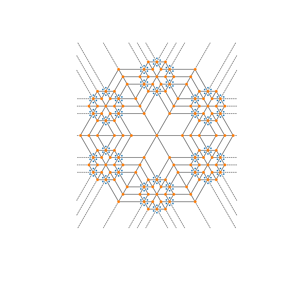
沃罗诺伊图可以用来创作有趣的创作艺术。尝试使用此设置 mandala 函数来创建您自己的!
>>> import numpy as np
>>> from scipy import spatial
>>> import matplotlib.pyplot as plt
>>> def mandala(n_iter, n_points, radius):
...     """Creates a mandala figure using Voronoi tesselations.
...
...     Parameters
...     ----------
...     n_iter : int
...         Number of iterations, i.e. how many times the equidistant points will
...         be generated.
...     n_points : int
...         Number of points to draw per iteration.
...     radius : scalar
...         The radial expansion factor.
...
...     Returns
...     -------
...     fig : matplotlib.Figure instance
...
...     Notes
...     -----
...     This code is adapted from the work of Audrey Roy Greenfeld [1]_ and Carlos
...     Focil-Espinosa [2]_, who created beautiful mandalas with Python code.  That
...     code in turn was based on Antonio Sánchez Chinchón's R code [3]_.
...
...     References
...     ----------
...     .. [1] https://www.codemakesmehappy.com/2019/09/voronoi-mandalas.html
...
...     .. [2] https://github.com/CarlosFocil/mandalapy
...
...     .. [3] https://github.com/aschinchon/mandalas
...
...     """
...     fig = plt.figure(figsize=(10, 10))
...     ax = fig.add_subplot(111)
...     ax.set_axis_off()
...     ax.set_aspect('equal', adjustable='box')
...
...     angles = np.linspace(0, 2*np.pi * (1 - 1/n_points), num=n_points) + np.pi/2
...     # Starting from a single center point, add points iteratively
...     xy = np.array([[0, 0]])
...     for k in range(n_iter):
...         t1 = np.array([])
...         t2 = np.array([])
...         # Add `n_points` new points around each existing point in this iteration
...         for i in range(xy.shape[0]):
...             t1 = np.append(t1, xy[i, 0] + radius**k * np.cos(angles))
...             t2 = np.append(t2, xy[i, 1] + radius**k * np.sin(angles))
...
...         xy = np.column_stack((t1, t2))
...
...     # Create the Mandala figure via a Voronoi plot
...     spatial.voronoi_plot_2d(spatial.Voronoi(xy), ax=ax)
...
...     return fig
>>> # Modify the following parameters in order to get different figures
>>> n_iter = 3
>>> n_points = 6
>>> radius = 4
>>> fig = mandala(n_iter, n_points, radius)
>>> plt.show()