重塑和透视表#
通过旋转DataFrame对象进行整形#
数据通常以所谓的“堆叠”或“记录”格式存储:
In [1]: import pandas._testing as tm

In [2]: def unpivot(frame):
   ...:     N, K = frame.shape
   ...:     data = {
   ...:         "value": frame.to_numpy().ravel("F"),
   ...:         "variable": np.asarray(frame.columns).repeat(N),
   ...:         "date": np.tile(np.asarray(frame.index), K),
   ...:     }
   ...:     return pd.DataFrame(data, columns=["date", "variable", "value"])
   ...:

In [3]: df = unpivot(tm.makeTimeDataFrame(3))

In [4]: df
Out[4]:
         date variable     value
0  2000-01-03        A  0.469112
1  2000-01-04        A -0.282863
2  2000-01-05        A -1.509059
3  2000-01-03        B -1.135632
4  2000-01-04        B  1.212112
5  2000-01-05        B -0.173215
6  2000-01-03        C  0.119209
7  2000-01-04        C -1.044236
8  2000-01-05        C -0.861849
9  2000-01-03        D -2.104569
10 2000-01-04        D -0.494929
11 2000-01-05        D  1.071804
为变量选择所有内容 A 我们可以这样做:
In [5]: filtered = df[df["variable"] == "A"]

In [6]: filtered
Out[6]:
        date variable     value
0 2000-01-03        A  0.469112
1 2000-01-04        A -0.282863
2 2000-01-05        A -1.509059
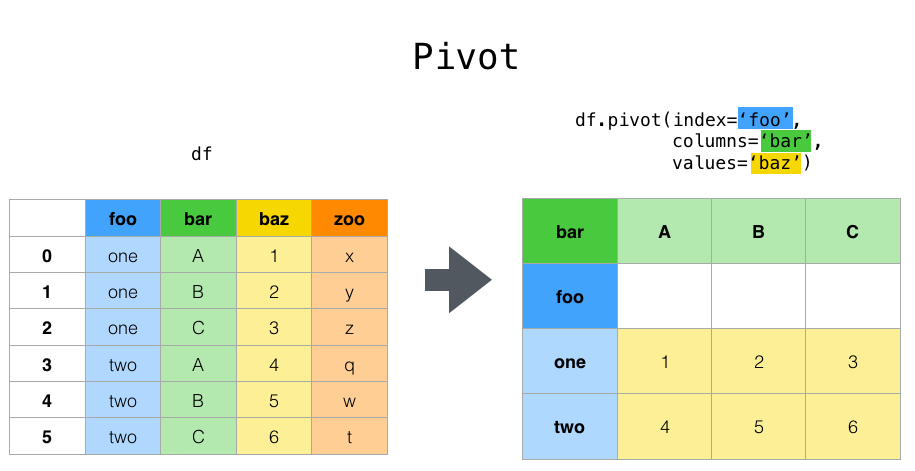
但假设我们希望对变量进行时间序列运算。更好的表现应该是 columns 是唯一的变量和 index 日期确定个人的观察结果。要将数据重塑为此表单,我们使用 DataFrame.pivot() 方法(也实现为顶级函数 pivot() ):
In [7]: pivoted = df.pivot(index="date", columns="variable", values="value")

In [8]: pivoted
Out[8]:
variable           A         B         C         D
date
2000-01-03  0.469112 -1.135632  0.119209 -2.104569
2000-01-04 -0.282863  1.212112 -1.044236 -0.494929
2000-01-05 -1.509059 -0.173215 -0.861849  1.071804
如果 values 参数被省略,并且输入 DataFrame 具有不用作列或索引输入的多列值 pivot() ,那么由此产生的“旋转” DataFrame 将会有 hierarchical columns 其最高级别表示各自的值列:
In [9]: df["value2"] = df["value"] * 2

In [10]: pivoted = df.pivot(index="date", columns="variable")

In [11]: pivoted
Out[11]:
               value                                  value2
variable           A         B         C         D         A         B         C         D
date
2000-01-03  0.469112 -1.135632  0.119209 -2.104569  0.938225 -2.271265  0.238417 -4.209138
2000-01-04 -0.282863  1.212112 -1.044236 -0.494929 -0.565727  2.424224 -2.088472 -0.989859
2000-01-05 -1.509059 -0.173215 -0.861849  1.071804 -3.018117 -0.346429 -1.723698  2.143608
然后,您可以从旋转的 DataFrame :
In [12]: pivoted["value2"]
Out[12]:
variable           A         B         C         D
date
2000-01-03  0.938225 -2.271265  0.238417 -4.209138
2000-01-04 -0.565727  2.424224 -2.088472 -0.989859
2000-01-05 -3.018117 -0.346429 -1.723698  2.143608
请注意,在数据是同构类型的情况下,这将返回底层数据的视图。
备注
pivot() 将使用 ValueError: Index contains duplicate entries, cannot reshape 如果索引/列对不是唯一的。在这种情况下,可以考虑使用 pivot_table() 它是PIVOT的泛化,可以处理一个索引/列对的重复值。
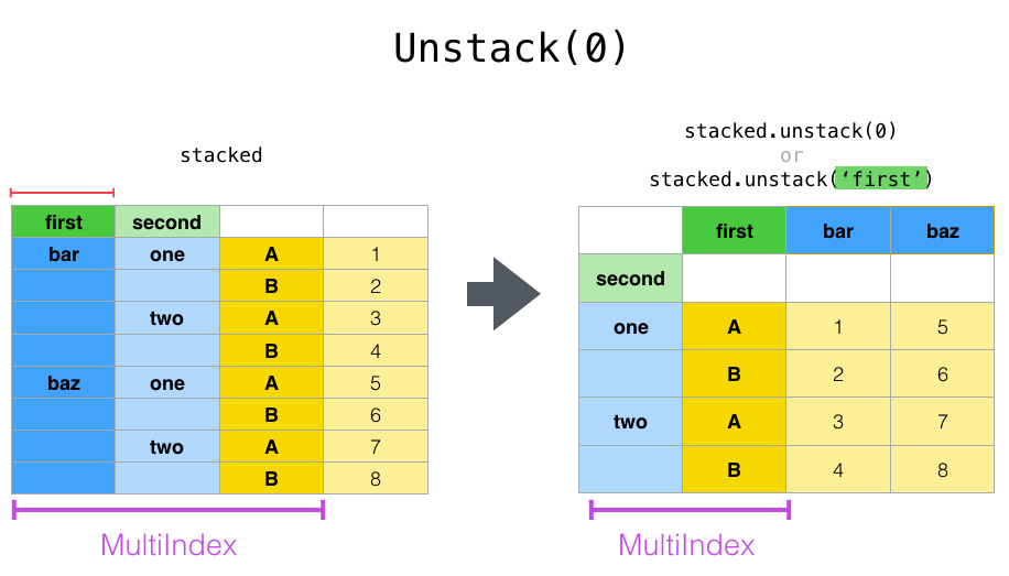
通过堆叠和取消堆叠来重塑#
与此密切相关 pivot() 方法是相关的 stack() 和 unstack() 上提供的方法 Series 和 DataFrame 。这些方法旨在与 MultiIndex 对象(请参阅 hierarchical indexing )。以下是这些方法的基本功能:
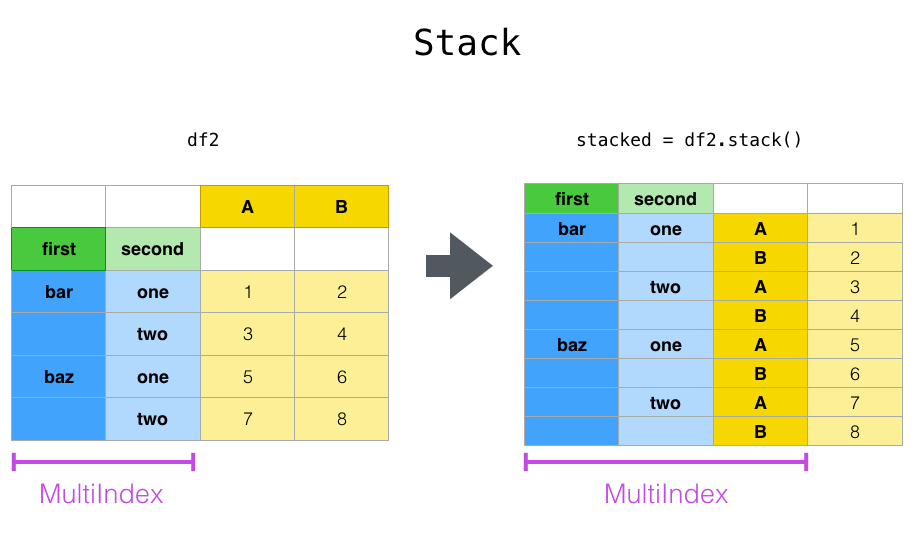
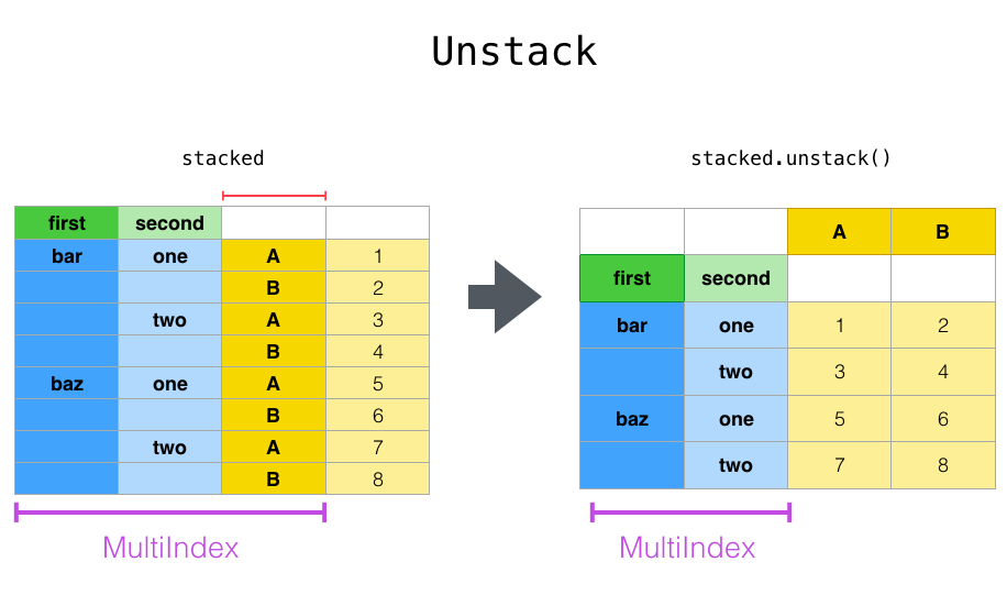
stack():“Pivot”列标签的一个级别(可能是分层的),返回一个DataFrame具有具有新的最内层行标签的索引。unstack():(逆运算stack())将行索引的一级(可能是分层的)“透视”到列轴,从而产生重塑的DataFrame具有新的最内层的列标签。
最清晰的解释方式就是举一反三。让我们以前面的层次索引部分中的一个示例数据集为例:
In [13]: tuples = list(
   ....:     zip(
   ....:         *[
   ....:             ["bar", "bar", "baz", "baz", "foo", "foo", "qux", "qux"],
   ....:             ["one", "two", "one", "two", "one", "two", "one", "two"],
   ....:         ]
   ....:     )
   ....: )
   ....:

In [14]: index = pd.MultiIndex.from_tuples(tuples, names=["first", "second"])

In [15]: df = pd.DataFrame(np.random.randn(8, 2), index=index, columns=["A", "B"])

In [16]: df2 = df[:4]

In [17]: df2
Out[17]:
                     A         B
first second
bar   one     0.721555 -0.706771
      two    -1.039575  0.271860
baz   one    -0.424972  0.567020
      two     0.276232 -1.087401
这个 stack() 函数将“压缩” DataFrame 用于产生以下任一结果的列:
A
Series,在简单列索引的情况下。A
DataFrame的情况下,MultiIndex在栏目里。
如果这些列具有 MultiIndex ,您可以选择要堆叠的级别。堆叠的级别将成为 MultiIndex 在各栏上:
In [18]: stacked = df2.stack()

In [19]: stacked
Out[19]:
first  second
bar    one     A    0.721555
               B   -0.706771
       two     A   -1.039575
               B    0.271860
baz    one     A   -0.424972
               B    0.567020
       two     A    0.276232
               B   -1.087401
dtype: float64
用一个“堆叠的” DataFrame 或 Series (有一个 MultiIndex 作为 index )的逆运算。 stack() 是 unstack() ,这在默认情况下会将 最后一关 :
In [20]: stacked.unstack()
Out[20]:
                     A         B
first second
bar   one     0.721555 -0.706771
      two    -1.039575  0.271860
baz   one    -0.424972  0.567020
      two     0.276232 -1.087401

In [21]: stacked.unstack(1)
Out[21]:
second        one       two
first
bar   A  0.721555 -1.039575
      B -0.706771  0.271860
baz   A -0.424972  0.276232
      B  0.567020 -1.087401

In [22]: stacked.unstack(0)
Out[22]:
first          bar       baz
second
one    A  0.721555 -0.424972
       B -0.706771  0.567020
two    A -1.039575  0.276232
       B  0.271860 -1.087401
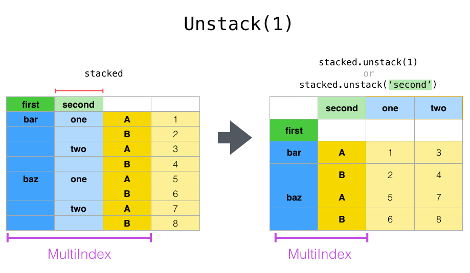
如果索引有名称,则可以使用级别名称,而不是指定级别编号:
In [23]: stacked.unstack("second")
Out[23]:
second        one       two
first
bar   A  0.721555 -1.039575
      B -0.706771  0.271860
baz   A -0.424972  0.276232
      B  0.567020 -1.087401
请注意, stack() 和 unstack() 方法隐式地对所涉及的索引级别进行排序。因此,呼吁 stack() 然后 unstack() ,或反之亦然,将导致 排序 原件复印件 DataFrame 或 Series :
In [24]: index = pd.MultiIndex.from_product([[2, 1], ["a", "b"]])

In [25]: df = pd.DataFrame(np.random.randn(4), index=index, columns=["A"])

In [26]: df
Out[26]:
            A
2 a -0.370647
  b -1.157892
1 a -1.344312
  b  0.844885

In [27]: all(df.unstack().stack() == df.sort_index())
Out[27]: True
上面的代码将引发一个 TypeError 如果调用 sort_index() 被移除。
多层次#
您还可以通过传递级别列表来一次堆叠或拆分多个级别,在这种情况下,最终结果就好像列表中的每个级别都是单独处理的一样。
In [28]: columns = pd.MultiIndex.from_tuples(
   ....:     [
   ....:         ("A", "cat", "long"),
   ....:         ("B", "cat", "long"),
   ....:         ("A", "dog", "short"),
   ....:         ("B", "dog", "short"),
   ....:     ],
   ....:     names=["exp", "animal", "hair_length"],
   ....: )
   ....:

In [29]: df = pd.DataFrame(np.random.randn(4, 4), columns=columns)

In [30]: df
Out[30]:
exp                 A         B         A         B
animal            cat       cat       dog       dog
hair_length      long      long     short     short
0            1.075770 -0.109050  1.643563 -1.469388
1            0.357021 -0.674600 -1.776904 -0.968914
2           -1.294524  0.413738  0.276662 -0.472035
3           -0.013960 -0.362543 -0.006154 -0.923061

In [31]: df.stack(level=["animal", "hair_length"])
Out[31]:
exp                          A         B
  animal hair_length
0 cat    long         1.075770 -0.109050
  dog    short        1.643563 -1.469388
1 cat    long         0.357021 -0.674600
  dog    short       -1.776904 -0.968914
2 cat    long        -1.294524  0.413738
  dog    short        0.276662 -0.472035
3 cat    long        -0.013960 -0.362543
  dog    short       -0.006154 -0.923061
标高列表可以包含标高名称或标高编号(但不能同时包含两者)。
# df.stack(level=['animal', 'hair_length'])
# from above is equivalent to:
In [32]: df.stack(level=[1, 2])
Out[32]:
exp                          A         B
  animal hair_length
0 cat    long         1.075770 -0.109050
  dog    short        1.643563 -1.469388
1 cat    long         0.357021 -0.674600
  dog    short       -1.776904 -0.968914
2 cat    long        -1.294524  0.413738
  dog    short        0.276662 -0.472035
3 cat    long        -0.013960 -0.362543
  dog    short       -0.006154 -0.923061
缺少数据#
这些函数对于处理丢失的数据是智能的,并且不期望分层索引中的每个子组具有相同的标签集。它们还可以处理未排序的索引(但您可以通过调用 sort_index() 当然)。下面是一个更复杂的例子:
In [33]: columns = pd.MultiIndex.from_tuples(
   ....:     [
   ....:         ("A", "cat"),
   ....:         ("B", "dog"),
   ....:         ("B", "cat"),
   ....:         ("A", "dog"),
   ....:     ],
   ....:     names=["exp", "animal"],
   ....: )
   ....:

In [34]: index = pd.MultiIndex.from_product(
   ....:     [("bar", "baz", "foo", "qux"), ("one", "two")], names=["first", "second"]
   ....: )
   ....:

In [35]: df = pd.DataFrame(np.random.randn(8, 4), index=index, columns=columns)

In [36]: df2 = df.iloc[[0, 1, 2, 4, 5, 7]]

In [37]: df2
Out[37]:
exp                  A         B                   A
animal             cat       dog       cat       dog
first second
bar   one     0.895717  0.805244 -1.206412  2.565646
      two     1.431256  1.340309 -1.170299 -0.226169
baz   one     0.410835  0.813850  0.132003 -0.827317
foo   one    -1.413681  1.607920  1.024180  0.569605
      two     0.875906 -2.211372  0.974466 -2.006747
qux   two    -1.226825  0.769804 -1.281247 -0.727707
如上所述, stack() 可以使用 level 参数选择要堆叠的列中的哪个级别:
In [38]: df2.stack("exp")
Out[38]:
animal                 cat       dog
first second exp
bar   one    A    0.895717  2.565646
             B   -1.206412  0.805244
      two    A    1.431256 -0.226169
             B   -1.170299  1.340309
baz   one    A    0.410835 -0.827317
             B    0.132003  0.813850
foo   one    A   -1.413681  0.569605
             B    1.024180  1.607920
      two    A    0.875906 -2.006747
             B    0.974466 -2.211372
qux   two    A   -1.226825 -0.727707
             B   -1.281247  0.769804

In [39]: df2.stack("animal")
Out[39]:
exp                         A         B
first second animal
bar   one    cat     0.895717 -1.206412
             dog     2.565646  0.805244
      two    cat     1.431256 -1.170299
             dog    -0.226169  1.340309
baz   one    cat     0.410835  0.132003
             dog    -0.827317  0.813850
foo   one    cat    -1.413681  1.024180
             dog     0.569605  1.607920
      two    cat     0.875906  0.974466
             dog    -2.006747 -2.211372
qux   two    cat    -1.226825 -1.281247
             dog    -0.727707  0.769804
如果子组不具有相同的标签集,则取消堆叠可能会导致缺少值。默认情况下,缺少的值将被该数据类型的默认填充值替换, NaN 对于浮动, NaT 对于类似日期的类型,等等。对于整型类型,默认情况下,数据将转换为浮点型,缺少的值将设置为 NaN 。
In [40]: df3 = df.iloc[[0, 1, 4, 7], [1, 2]]

In [41]: df3
Out[41]:
exp                  B
animal             dog       cat
first second
bar   one     0.805244 -1.206412
      two     1.340309 -1.170299
foo   one     1.607920  1.024180
qux   two     0.769804 -1.281247

In [42]: df3.unstack()
Out[42]:
exp            B
animal       dog                 cat
second       one       two       one       two
first
bar     0.805244  1.340309 -1.206412 -1.170299
foo     1.607920       NaN  1.024180       NaN
qux          NaN  0.769804       NaN -1.281247
或者,取消堆栈需要一个可选的 fill_value 参数,用于指定缺失数据的值。
In [43]: df3.unstack(fill_value=-1e9)
Out[43]:
exp                B
animal           dog                         cat
second           one           two           one           two
first
bar     8.052440e-01  1.340309e+00 -1.206412e+00 -1.170299e+00
foo     1.607920e+00 -1.000000e+09  1.024180e+00 -1.000000e+09
qux    -1.000000e+09  7.698036e-01 -1.000000e+09 -1.281247e+00
使用多索引#
当柱是 MultiIndex 在做正确的事情时也很谨慎:
In [44]: df[:3].unstack(0)
Out[44]:
exp            A                   B                                      A
animal       cat                 dog                cat                 dog
first        bar       baz       bar      baz       bar       baz       bar       baz
second
one     0.895717  0.410835  0.805244  0.81385 -1.206412  0.132003  2.565646 -0.827317
two     1.431256       NaN  1.340309      NaN -1.170299       NaN -0.226169       NaN

In [45]: df2.unstack(1)
Out[45]:
exp            A                   B                                       A
animal       cat                 dog                 cat                 dog
second       one       two       one       two       one       two       one       two
first
bar     0.895717  1.431256  0.805244  1.340309 -1.206412 -1.170299  2.565646 -0.226169
baz     0.410835       NaN  0.813850       NaN  0.132003       NaN -0.827317       NaN
foo    -1.413681  0.875906  1.607920 -2.211372  1.024180  0.974466  0.569605 -2.006747
qux          NaN -1.226825       NaN  0.769804       NaN -1.281247       NaN -0.727707
熔化重塑#
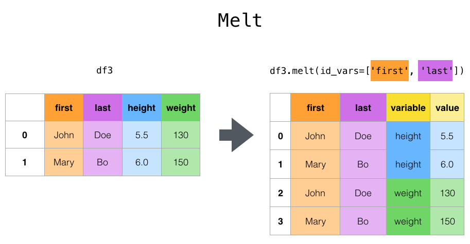
最高层 melt() 函数和相应的 DataFrame.melt() 对按摩一个人很有用 DataFrame 转换为一列或多列的格式 标识符变量 ,而所有其他列,则考虑 测量变量 “不旋转”到行轴,只剩下两个非标识符列“Variable”和“Value”。这些列的名称可以通过提供 var_name 和 value_name 参数。
例如,
In [46]: cheese = pd.DataFrame(
   ....:     {
   ....:         "first": ["John", "Mary"],
   ....:         "last": ["Doe", "Bo"],
   ....:         "height": [5.5, 6.0],
   ....:         "weight": [130, 150],
   ....:     }
   ....: )
   ....:

In [47]: cheese
Out[47]:
  first last  height  weight
0  John  Doe     5.5     130
1  Mary   Bo     6.0     150

In [48]: cheese.melt(id_vars=["first", "last"])
Out[48]:
  first last variable  value
0  John  Doe   height    5.5
1  Mary   Bo   height    6.0
2  John  Doe   weight  130.0
3  Mary   Bo   weight  150.0

In [49]: cheese.melt(id_vars=["first", "last"], var_name="quantity")
Out[49]:
  first last quantity  value
0  John  Doe   height    5.5
1  Mary   Bo   height    6.0
2  John  Doe   weight  130.0
3  Mary   Bo   weight  150.0
使用转换DataFrame时 melt() ,则该索引将被忽略。属性可以保留原始索引值。 ignore_index 参数设置为 False (默认为 True )。然而,这将复制它们。
1.1.0 新版功能.
In [50]: index = pd.MultiIndex.from_tuples([("person", "A"), ("person", "B")])

In [51]: cheese = pd.DataFrame(
   ....:     {
   ....:         "first": ["John", "Mary"],
   ....:         "last": ["Doe", "Bo"],
   ....:         "height": [5.5, 6.0],
   ....:         "weight": [130, 150],
   ....:     },
   ....:     index=index,
   ....: )
   ....:

In [52]: cheese
Out[52]:
         first last  height  weight
person A  John  Doe     5.5     130
       B  Mary   Bo     6.0     150

In [53]: cheese.melt(id_vars=["first", "last"])
Out[53]:
  first last variable  value
0  John  Doe   height    5.5
1  Mary   Bo   height    6.0
2  John  Doe   weight  130.0
3  Mary   Bo   weight  150.0

In [54]: cheese.melt(id_vars=["first", "last"], ignore_index=False)
Out[54]:
         first last variable  value
person A  John  Doe   height    5.5
       B  Mary   Bo   height    6.0
       A  John  Doe   weight  130.0
       B  Mary   Bo   weight  150.0
另一种转换方法是使用 wide_to_long() 面板数据便捷功能。它的灵活性不如 melt() ,但更人性化。
In [55]: dft = pd.DataFrame(
   ....:     {
   ....:         "A1970": {0: "a", 1: "b", 2: "c"},
   ....:         "A1980": {0: "d", 1: "e", 2: "f"},
   ....:         "B1970": {0: 2.5, 1: 1.2, 2: 0.7},
   ....:         "B1980": {0: 3.2, 1: 1.3, 2: 0.1},
   ....:         "X": dict(zip(range(3), np.random.randn(3))),
   ....:     }
   ....: )
   ....:

In [56]: dft["id"] = dft.index

In [57]: dft
Out[57]:
  A1970 A1980  B1970  B1980         X  id
0     a     d    2.5    3.2 -0.121306   0
1     b     e    1.2    1.3 -0.097883   1
2     c     f    0.7    0.1  0.695775   2

In [58]: pd.wide_to_long(dft, ["A", "B"], i="id", j="year")
Out[58]:
                X  A    B
id year
0  1970 -0.121306  a  2.5
1  1970 -0.097883  b  1.2
2  1970  0.695775  c  0.7
0  1980 -0.121306  d  3.2
1  1980 -0.097883  e  1.3
2  1980  0.695775  f  0.1
与统计数据和分组依据相结合#
结合在一起应该不会令人震惊 pivot() / stack() / unstack() 使用GroupBy以及Basic Series和DataFrame,统计函数可以产生一些非常有表现力的快速数据操作。
In [59]: df
Out[59]:
exp                  A         B                   A
animal             cat       dog       cat       dog
first second
bar   one     0.895717  0.805244 -1.206412  2.565646
      two     1.431256  1.340309 -1.170299 -0.226169
baz   one     0.410835  0.813850  0.132003 -0.827317
      two    -0.076467 -1.187678  1.130127 -1.436737
foo   one    -1.413681  1.607920  1.024180  0.569605
      two     0.875906 -2.211372  0.974466 -2.006747
qux   one    -0.410001 -0.078638  0.545952 -1.219217
      two    -1.226825  0.769804 -1.281247 -0.727707

In [60]: df.stack().mean(1).unstack()
Out[60]:
animal             cat       dog
first second
bar   one    -0.155347  1.685445
      two     0.130479  0.557070
baz   one     0.271419 -0.006733
      two     0.526830 -1.312207
foo   one    -0.194750  1.088763
      two     0.925186 -2.109060
qux   one     0.067976 -0.648927
      two    -1.254036  0.021048

# same result, another way
In [61]: df.groupby(level=1, axis=1).mean()
Out[61]:
animal             cat       dog
first second
bar   one    -0.155347  1.685445
      two     0.130479  0.557070
baz   one     0.271419 -0.006733
      two     0.526830 -1.312207
foo   one    -0.194750  1.088763
      two     0.925186 -2.109060
qux   one     0.067976 -0.648927
      two    -1.254036  0.021048

In [62]: df.stack().groupby(level=1).mean()
Out[62]:
exp            A         B
second
one     0.071448  0.455513
two    -0.424186 -0.204486

In [63]: df.mean().unstack(0)
Out[63]:
exp            A         B
animal
cat     0.060843  0.018596
dog    -0.413580  0.232430
数据透视表#
而当 pivot() 提供具有各种数据类型(字符串、数字等)的通用透视,PANAS还提供 pivot_table() 用于使用数字数据聚合进行透视。
该函数 pivot_table() 可用于创建电子表格样式的数据透视表。请参阅 cookbook 一些先进的策略。
它需要一些论据:
data:DataFrame对象。values:要聚合的一列或一列。index:与数据长度相同的列、Grouper、数组或它们的列表。透视表索引上分组依据的键。如果传递数组,则它的使用方式与列值相同。columns:与数据长度相同的列、Grouper、数组或它们的列表。透视表表列上分组依据的键。如果传递数组,则它的使用方式与列值相同。aggfunc:用于聚合的函数,默认为numpy.mean。
考虑如下数据集:
In [64]: import datetime

In [65]: df = pd.DataFrame(
   ....:     {
   ....:         "A": ["one", "one", "two", "three"] * 6,
   ....:         "B": ["A", "B", "C"] * 8,
   ....:         "C": ["foo", "foo", "foo", "bar", "bar", "bar"] * 4,
   ....:         "D": np.random.randn(24),
   ....:         "E": np.random.randn(24),
   ....:         "F": [datetime.datetime(2013, i, 1) for i in range(1, 13)]
   ....:         + [datetime.datetime(2013, i, 15) for i in range(1, 13)],
   ....:     }
   ....: )
   ....:

In [66]: df
Out[66]:
        A  B    C         D         E          F
0     one  A  foo  0.341734 -0.317441 2013-01-01
1     one  B  foo  0.959726 -1.236269 2013-02-01
2     two  C  foo -1.110336  0.896171 2013-03-01
3   three  A  bar -0.619976 -0.487602 2013-04-01
4     one  B  bar  0.149748 -0.082240 2013-05-01
..    ... ..  ...       ...       ...        ...
19  three  B  foo  0.690579 -2.213588 2013-08-15
20    one  C  foo  0.995761  1.063327 2013-09-15
21    one  A  bar  2.396780  1.266143 2013-10-15
22    two  B  bar  0.014871  0.299368 2013-11-15
23  three  C  bar  3.357427 -0.863838 2013-12-15

[24 rows x 6 columns]
我们可以非常容易地从这些数据生成数据透视表:
In [67]: pd.pivot_table(df, values="D", index=["A", "B"], columns=["C"])
Out[67]:
C             bar       foo
A     B
one   A  1.120915 -0.514058
      B -0.338421  0.002759
      C -0.538846  0.699535
three A -1.181568       NaN
      B       NaN  0.433512
      C  0.588783       NaN
two   A       NaN  1.000985
      B  0.158248       NaN
      C       NaN  0.176180

In [68]: pd.pivot_table(df, values="D", index=["B"], columns=["A", "C"], aggfunc=np.sum)
Out[68]:
A       one               three                 two
C       bar       foo       bar       foo       bar       foo
B
A  2.241830 -1.028115 -2.363137       NaN       NaN  2.001971
B -0.676843  0.005518       NaN  0.867024  0.316495       NaN
C -1.077692  1.399070  1.177566       NaN       NaN  0.352360

In [69]: pd.pivot_table(
   ....:     df, values=["D", "E"],
   ....:     index=["B"],
   ....:     columns=["A", "C"],
   ....:     aggfunc=np.sum,
   ....: )
   ....:
Out[69]:
          D                                                           E
A       one               three                 two                 one               three                 two
C       bar       foo       bar       foo       bar       foo       bar       foo       bar       foo       bar       foo
B
A  2.241830 -1.028115 -2.363137       NaN       NaN  2.001971  2.786113 -0.043211  1.922577       NaN       NaN  0.128491
B -0.676843  0.005518       NaN  0.867024  0.316495       NaN  1.368280 -1.103384       NaN -2.128743 -0.194294       NaN
C -1.077692  1.399070  1.177566       NaN       NaN  0.352360 -1.976883  1.495717 -0.263660       NaN       NaN  0.872482
结果对象是一个 DataFrame 在行和列上具有潜在的分层索引。如果 values 如果未指定列名,则数据透视表将包括可以在列中的其他层次结构级别中聚合的所有数据:
In [70]: pd.pivot_table(df, index=["A", "B"], columns=["C"])
Out[70]:
                D                   E
C             bar       foo       bar       foo
A     B
one   A  1.120915 -0.514058  1.393057 -0.021605
      B -0.338421  0.002759  0.684140 -0.551692
      C -0.538846  0.699535 -0.988442  0.747859
three A -1.181568       NaN  0.961289       NaN
      B       NaN  0.433512       NaN -1.064372
      C  0.588783       NaN -0.131830       NaN
two   A       NaN  1.000985       NaN  0.064245
      B  0.158248       NaN -0.097147       NaN
      C       NaN  0.176180       NaN  0.436241
此外,您还可以使用 Grouper 为 index 和 columns 关键字。有关详情,请参阅 Grouper ,请参见 Grouping with a Grouper specification 。
In [71]: pd.pivot_table(df, values="D", index=pd.Grouper(freq="M", key="F"), columns="C")
Out[71]:
C                bar       foo
F
2013-01-31       NaN -0.514058
2013-02-28       NaN  0.002759
2013-03-31       NaN  0.176180
2013-04-30 -1.181568       NaN
2013-05-31 -0.338421       NaN
2013-06-30 -0.538846       NaN
2013-07-31       NaN  1.000985
2013-08-31       NaN  0.433512
2013-09-30       NaN  0.699535
2013-10-31  1.120915       NaN
2013-11-30  0.158248       NaN
2013-12-31  0.588783       NaN
您可以通过调用以下方法呈现一个很好的表输出,省略缺少的值 to_string() 如果您愿意:
In [72]: table = pd.pivot_table(df, index=["A", "B"], columns=["C"])

In [73]: print(table.to_string(na_rep=""))
                D                   E
C             bar       foo       bar       foo
A     B
one   A  1.120915 -0.514058  1.393057 -0.021605
      B -0.338421  0.002759  0.684140 -0.551692
      C -0.538846  0.699535 -0.988442  0.747859
three A -1.181568            0.961289
      B            0.433512           -1.064372
      C  0.588783           -0.131830
two   A            1.000985            0.064245
      B  0.158248           -0.097147
      C            0.176180            0.436241
- 请注意,
pivot_table()也可作为DataFrame上的实例方法使用,
添加页边距#
如果你通过了 margins=True 至 pivot_table() ,特别 All 将在行和列的类别中添加具有部分组聚合的列和行:
In [74]: table = df.pivot_table(index=["A", "B"], columns="C", margins=True, aggfunc=np.std)

In [75]: table
Out[75]:
                D                             E
C             bar       foo       All       bar       foo       All
A     B
one   A  1.804346  1.210272  1.569879  0.179483  0.418374  0.858005
      B  0.690376  1.353355  0.898998  1.083825  0.968138  1.101401
      C  0.273641  0.418926  0.771139  1.689271  0.446140  1.422136
three A  0.794212       NaN  0.794212  2.049040       NaN  2.049040
      B       NaN  0.363548  0.363548       NaN  1.625237  1.625237
      C  3.915454       NaN  3.915454  1.035215       NaN  1.035215
two   A       NaN  0.442998  0.442998       NaN  0.447104  0.447104
      B  0.202765       NaN  0.202765  0.560757       NaN  0.560757
      C       NaN  1.819408  1.819408       NaN  0.650439  0.650439
All      1.556686  0.952552  1.246608  1.250924  0.899904  1.059389
此外,您还可以调用 DataFrame.stack() 要将已透视的DataFrame显示为具有多级索引,请执行以下操作:
In [76]: table.stack()
Out[76]:
                  D         E
A   B C
one A All  1.569879  0.858005
      bar  1.804346  0.179483
      foo  1.210272  0.418374
    B All  0.898998  1.101401
      bar  0.690376  1.083825
...             ...       ...
two C All  1.819408  0.650439
      foo  1.819408  0.650439
All   All  1.246608  1.059389
      bar  1.556686  1.250924
      foo  0.952552  0.899904

[24 rows x 2 columns]
交叉表#
使用 crosstab() 计算两个(或多个)因素的交叉表。默认情况下 crosstab() 除非传递了值数组和聚合函数,否则计算因子的频率表。
它需要许多论据
index:类似于数组的行中分组依据的值。columns:类似数组的值,列中的分组依据。values:数组形式,可选,根据系数聚合的值数组。aggfunc:函数,可选,如果没有传递任何值数组,则计算频率表。rownames:序列,默认None必须与传递的行数组数目匹配。colnames:序列,默认None如果传递,则必须与传递的列数组数目匹配。margins:布尔值,默认False,添加行/列边距(小计)normalize: boolean, {'all', 'index', 'columns'}, or {0,1}, defaultFalse. Normalize by dividing all values by the sum of values.
任何 Series 除非指定了交叉表的行名或列名,否则将使用传递的名称属性
例如:
In [77]: foo, bar, dull, shiny, one, two = "foo", "bar", "dull", "shiny", "one", "two"

In [78]: a = np.array([foo, foo, bar, bar, foo, foo], dtype=object)

In [79]: b = np.array([one, one, two, one, two, one], dtype=object)

In [80]: c = np.array([dull, dull, shiny, dull, dull, shiny], dtype=object)

In [81]: pd.crosstab(a, [b, c], rownames=["a"], colnames=["b", "c"])
Out[81]:
b    one        two
c   dull shiny dull shiny
a
bar    1     0    0     1
foo    2     1    1     0
如果 crosstab() 只接收两个系列,它将提供频率表。
In [82]: df = pd.DataFrame(
   ....:     {"A": [1, 2, 2, 2, 2], "B": [3, 3, 4, 4, 4], "C": [1, 1, np.nan, 1, 1]}
   ....: )
   ....:

In [83]: df
Out[83]:
   A  B    C
0  1  3  1.0
1  2  3  1.0
2  2  4  NaN
3  2  4  1.0
4  2  4  1.0

In [84]: pd.crosstab(df["A"], df["B"])
Out[84]:
B  3  4
A
1  1  0
2  1  3
crosstab() 也可以实现为 Categorical 数据。
In [85]: foo = pd.Categorical(["a", "b"], categories=["a", "b", "c"])

In [86]: bar = pd.Categorical(["d", "e"], categories=["d", "e", "f"])

In [87]: pd.crosstab(foo, bar)
Out[87]:
col_0  d  e
row_0
a      1  0
b      0  1
如果您想包括 all 即使实际数据不包含特定类别的任何实例,也应设置 dropna=False 。
例如:
In [88]: pd.crosstab(foo, bar, dropna=False)
Out[88]:
col_0  d  e  f
row_0
a      1  0  0
b      0  1  0
c      0  0  0
正规化#
还可以标准化频率表以显示百分比,而不是使用 normalize 论点:
In [89]: pd.crosstab(df["A"], df["B"], normalize=True)
Out[89]:
B    3    4
A
1  0.2  0.0
2  0.2  0.6
normalize 还可以规格化每行或每列中的值:
In [90]: pd.crosstab(df["A"], df["B"], normalize="columns")
Out[90]:
B    3    4
A
1  0.5  0.0
2  0.5  1.0
crosstab() 也可以通过第三个 Series 和聚合函数 (aggfunc ),它将应用于第三个 Series 在由前两个定义的每个组中 Series :
In [91]: pd.crosstab(df["A"], df["B"], values=df["C"], aggfunc=np.sum)
Out[91]:
B    3    4
A
1  1.0  NaN
2  1.0  2.0
添加页边距#
最后,还可以增加页边距或将此输出正常化。
In [92]: pd.crosstab(
   ....:     df["A"], df["B"], values=df["C"], aggfunc=np.sum, normalize=True, margins=True
   ....: )
   ....:
Out[92]:
B       3    4   All
A
1    0.25  0.0  0.25
2    0.25  0.5  0.75
All  0.50  0.5  1.00
贴瓷砖#
这个 cut() 函数计算输入数组的值的分组,通常用于将连续变量转换为离散变量或分类变量:
In [93]: ages = np.array([10, 15, 13, 12, 23, 25, 28, 59, 60])

In [94]: pd.cut(ages, bins=3)
Out[94]:
[(9.95, 26.667], (9.95, 26.667], (9.95, 26.667], (9.95, 26.667], (9.95, 26.667], (9.95, 26.667], (26.667, 43.333], (43.333, 60.0], (43.333, 60.0]]
Categories (3, interval[float64, right]): [(9.95, 26.667] < (26.667, 43.333] < (43.333, 60.0]]
如果 bins 关键字为整数,则形成等宽仓位。或者,我们可以指定定制的边框边缘:
In [95]: c = pd.cut(ages, bins=[0, 18, 35, 70])

In [96]: c
Out[96]:
[(0, 18], (0, 18], (0, 18], (0, 18], (18, 35], (18, 35], (18, 35], (35, 70], (35, 70]]
Categories (3, interval[int64, right]): [(0, 18] < (18, 35] < (35, 70]]
如果 bins 关键字是一个 IntervalIndex ,则这些将用于将传递的数据入库。::
pd.cut([25, 20, 50], bins=c.categories)
计算指标/虚拟变量#
将类别变量转换为“哑元”或“指示符” DataFrame ,例如, DataFrame (A) Series ),它有 k 不同的值,可以派生一个 DataFrame 包含 k 使用1和0的列 get_dummies() :
In [97]: df = pd.DataFrame({"key": list("bbacab"), "data1": range(6)})

In [98]: pd.get_dummies(df["key"])
Out[98]:
   a  b  c
0  0  1  0
1  0  1  0
2  1  0  0
3  0  0  1
4  1  0  0
5  0  1  0
有时,在列名前面加上前缀很有用,例如,在将结果与原始结果合并时 DataFrame :
In [99]: dummies = pd.get_dummies(df["key"], prefix="key")

In [100]: dummies
Out[100]:
   key_a  key_b  key_c
0      0      1      0
1      0      1      0
2      1      0      0
3      0      0      1
4      1      0      0
5      0      1      0

In [101]: df[["data1"]].join(dummies)
Out[101]:
   data1  key_a  key_b  key_c
0      0      0      1      0
1      1      0      1      0
2      2      1      0      0
3      3      0      0      1
4      4      1      0      0
5      5      0      1      0
此函数通常与离散化函数一起使用,如 cut() :
In [102]: values = np.random.randn(10)

In [103]: values
Out[103]:
array([ 0.4082, -1.0481, -0.0257, -0.9884,  0.0941,  1.2627,  1.29  ,
        0.0824, -0.0558,  0.5366])

In [104]: bins = [0, 0.2, 0.4, 0.6, 0.8, 1]

In [105]: pd.get_dummies(pd.cut(values, bins))
Out[105]:
   (0.0, 0.2]  (0.2, 0.4]  (0.4, 0.6]  (0.6, 0.8]  (0.8, 1.0]
0           0           0           1           0           0
1           0           0           0           0           0
2           0           0           0           0           0
3           0           0           0           0           0
4           1           0           0           0           0
5           0           0           0           0           0
6           0           0           0           0           0
7           1           0           0           0           0
8           0           0           0           0           0
9           0           0           1           0           0
另请参阅 Series.str.get_dummies 。
get_dummies() 还接受一个 DataFrame 。默认情况下,所有类别变量(在统计意义上是类别变量,具有 object 或 categorical 数据类型)被编码为伪变量。
In [106]: df = pd.DataFrame({"A": ["a", "b", "a"], "B": ["c", "c", "b"], "C": [1, 2, 3]})

In [107]: pd.get_dummies(df)
Out[107]:
   C  A_a  A_b  B_b  B_c
0  1    1    0    0    1
1  2    0    1    0    1
2  3    1    0    1    0
所有非对象列都原封不动地包含在输出中。属性编码的列。 columns 关键字。
In [108]: pd.get_dummies(df, columns=["A"])
Out[108]:
   B  C  A_a  A_b
0  c  1    1    0
1  c  2    0    1
2  b  3    1    0
请注意, B 列仍包含在输出中,只是尚未编码。你可以放弃 B 在打电话之前 get_dummies 如果您不想将其包括在输出中。
就像 Series 版本,则可以将 prefix 和 prefix_sep 。缺省情况下,列名用作前缀,并且 _ 作为前缀分隔符。您可以指定 prefix 和 prefix_sep 在三个方面:
字符串:使用相同的值
prefix或prefix_sep对于要编码的每一列。List:长度必须与要编码的列数相同。
Dict:将列名映射到前缀。
In [109]: simple = pd.get_dummies(df, prefix="new_prefix")

In [110]: simple
Out[110]:
   C  new_prefix_a  new_prefix_b  new_prefix_b  new_prefix_c
0  1             1             0             0             1
1  2             0             1             0             1
2  3             1             0             1             0

In [111]: from_list = pd.get_dummies(df, prefix=["from_A", "from_B"])

In [112]: from_list
Out[112]:
   C  from_A_a  from_A_b  from_B_b  from_B_c
0  1         1         0         0         1
1  2         0         1         0         1
2  3         1         0         1         0

In [113]: from_dict = pd.get_dummies(df, prefix={"B": "from_B", "A": "from_A"})

In [114]: from_dict
Out[114]:
   C  from_A_a  from_A_b  from_B_b  from_B_c
0  1         1         0         0         1
1  2         0         1         0         1
2  3         1         0         1         0
有时,在将结果提供给统计模型时,仅保留分类变量的k-1个级别将是有用的,以避免共线性。您可以通过打开来切换到此模式 drop_first 。
In [115]: s = pd.Series(list("abcaa"))

In [116]: pd.get_dummies(s)
Out[116]:
   a  b  c
0  1  0  0
1  0  1  0
2  0  0  1
3  1  0  0
4  1  0  0

In [117]: pd.get_dummies(s, drop_first=True)
Out[117]:
   b  c
0  0  0
1  1  0
2  0  1
3  0  0
4  0  0
当一列只包含一个级别时,它将在结果中被省略。
In [118]: df = pd.DataFrame({"A": list("aaaaa"), "B": list("ababc")})

In [119]: pd.get_dummies(df)
Out[119]:
   A_a  B_a  B_b  B_c
0    1    1    0    0
1    1    0    1    0
2    1    1    0    0
3    1    0    1    0
4    1    0    0    1

In [120]: pd.get_dummies(df, drop_first=True)
Out[120]:
   B_b  B_c
0    0    0
1    1    0
2    0    0
3    1    0
4    0    1
默认情况下,新列将具有 np.uint8 数据类型。若要选择其他数据类型,请使用 dtype 论点:
In [121]: df = pd.DataFrame({"A": list("abc"), "B": [1.1, 2.2, 3.3]})

In [122]: pd.get_dummies(df, dtype=bool).dtypes
Out[122]:
B      float64
A_a       bool
A_b       bool
A_c       bool
dtype: object
因式分解值#
若要将1-d值编码为枚举类型,请使用 factorize() :
In [123]: x = pd.Series(["A", "A", np.nan, "B", 3.14, np.inf])

In [124]: x
Out[124]:
0       A
1       A
2     NaN
3       B
4    3.14
5     inf
dtype: object

In [125]: labels, uniques = pd.factorize(x)

In [126]: labels
Out[126]: array([ 0,  0, -1,  1,  2,  3])

In [127]: uniques
Out[127]: Index(['A', 'B', 3.14, inf], dtype='object')
请注意, factorize() 类似于 numpy.unique ,但在处理NaN方面有所不同:
备注
以下内容 numpy.unique will fail under Python 3 with a TypeError because of an ordering bug. See also here 。
In [128]: ser = pd.Series(['A', 'A', np.nan, 'B', 3.14, np.inf])

In [129]: pd.factorize(ser, sort=True)
Out[129]: (array([ 2,  2, -1,  3,  0,  1]), Index([3.14, inf, 'A', 'B'], dtype='object'))

In [130]: np.unique(ser, return_inverse=True)[::-1]
---------------------------------------------------------------------------
TypeError                                 Traceback (most recent call last)
Input In [130], in <cell line: 1>()
----> 1 np.unique(ser, return_inverse=True)[::-1]

File <__array_function__ internals>:5, in unique(*args, **kwargs)

File /usr/lib/python3/dist-packages/numpy/lib/arraysetops.py:272, in unique(ar, return_index, return_inverse, return_counts, axis)
    270 ar = np.asanyarray(ar)
    271 if axis is None:
--> 272     ret = _unique1d(ar, return_index, return_inverse, return_counts)
    273     return _unpack_tuple(ret)
    275 # axis was specified and not None

File /usr/lib/python3/dist-packages/numpy/lib/arraysetops.py:330, in _unique1d(ar, return_index, return_inverse, return_counts)
    327 optional_indices = return_index or return_inverse
    329 if optional_indices:
--> 330     perm = ar.argsort(kind='mergesort' if return_index else 'quicksort')
    331     aux = ar[perm]
    332 else:

TypeError: '<' not supported between instances of 'float' and 'str'
备注
如果您只想将一列作为分类变量(如R的因子)处理,则可以使用 df["cat_col"] = pd.Categorical(df["col"]) 或 df["cat_col"] = df["col"].astype("category") 。有关完整的文档,请访问 Categorical ,请参阅 Categorical introduction 以及 API documentation 。
示例#
在本节中,我们将复习常见问题和示例。在下面的答案中,列名和相关列值的命名与此DataFrame的透视方式相对应。
In [131]: np.random.seed([3, 1415])

In [132]: n = 20

In [133]: cols = np.array(["key", "row", "item", "col"])

In [134]: df = cols + pd.DataFrame(
   .....:     (np.random.randint(5, size=(n, 4)) // [2, 1, 2, 1]).astype(str)
   .....: )
   .....:

In [135]: df.columns = cols

In [136]: df = df.join(pd.DataFrame(np.random.rand(n, 2).round(2)).add_prefix("val"))

In [137]: df
Out[137]:
     key   row   item   col  val0  val1
0   key0  row3  item1  col3  0.81  0.04
1   key1  row2  item1  col2  0.44  0.07
2   key1  row0  item1  col0  0.77  0.01
3   key0  row4  item0  col2  0.15  0.59
4   key1  row0  item2  col1  0.81  0.64
..   ...   ...    ...   ...   ...   ...
15  key0  row3  item1  col1  0.31  0.23
16  key0  row0  item2  col3  0.86  0.01
17  key0  row4  item0  col3  0.64  0.21
18  key2  row2  item2  col0  0.13  0.45
19  key0  row2  item0  col4  0.37  0.70

[20 rows x 6 columns]
使用单个聚合进行旋转#
假设我们想要旋转 df 这样的话 col 值为列, row 值是索引,其平均值为 val0 是价值观吗?特别是,生成的DataFrame应该如下所示:
col   col0   col1   col2   col3  col4
row
row0  0.77  0.605    NaN  0.860  0.65
row2  0.13    NaN  0.395  0.500  0.25
row3   NaN  0.310    NaN  0.545   NaN
row4   NaN  0.100  0.395  0.760  0.24
此解决方案使用 pivot_table() 。另请注意, aggfunc='mean' 是默认设置。在这里包含它是为了明确。
In [138]: df.pivot_table(values="val0", index="row", columns="col", aggfunc="mean")
Out[138]:
col   col0   col1   col2   col3  col4
row
row0  0.77  0.605    NaN  0.860  0.65
row2  0.13    NaN  0.395  0.500  0.25
row3   NaN  0.310    NaN  0.545   NaN
row4   NaN  0.100  0.395  0.760  0.24
注意,我们还可以通过使用 fill_value 参数。
In [139]: df.pivot_table(
   .....:     values="val0",
   .....:     index="row",
   .....:     columns="col",
   .....:     aggfunc="mean",
   .....:     fill_value=0,
   .....: )
   .....:
Out[139]:
col   col0   col1   col2   col3  col4
row
row0  0.77  0.605  0.000  0.860  0.65
row2  0.13  0.000  0.395  0.500  0.25
row3  0.00  0.310  0.000  0.545  0.00
row4  0.00  0.100  0.395  0.760  0.24
还要注意,我们还可以传入其他聚合函数。例如,我们还可以传入 sum 。
In [140]: df.pivot_table(
   .....:     values="val0",
   .....:     index="row",
   .....:     columns="col",
   .....:     aggfunc="sum",
   .....:     fill_value=0,
   .....: )
   .....:
Out[140]:
col   col0  col1  col2  col3  col4
row
row0  0.77  1.21  0.00  0.86  0.65
row2  0.13  0.00  0.79  0.50  0.50
row3  0.00  0.31  0.00  1.09  0.00
row4  0.00  0.10  0.79  1.52  0.24
我们可以做的另一个聚合是计算列和行一起出现的频率。“交叉表”。要做到这一点,我们可以 size 发送到 aggfunc 参数。
In [141]: df.pivot_table(index="row", columns="col", fill_value=0, aggfunc="size")
Out[141]:
col   col0  col1  col2  col3  col4
row
row0     1     2     0     1     1
row2     1     0     2     1     2
row3     0     1     0     2     0
row4     0     1     2     2     1
使用多个聚合进行旋转#
我们还可以执行多个聚合。例如,要同时执行 sum 和 mean ,我们可以将列表传递给 aggfunc 论点。
In [142]: df.pivot_table(
   .....:     values="val0",
   .....:     index="row",
   .....:     columns="col",
   .....:     aggfunc=["mean", "sum"],
   .....: )
   .....:
Out[142]:
      mean                              sum
col   col0   col1   col2   col3  col4  col0  col1  col2  col3  col4
row
row0  0.77  0.605    NaN  0.860  0.65  0.77  1.21   NaN  0.86  0.65
row2  0.13    NaN  0.395  0.500  0.25  0.13   NaN  0.79  0.50  0.50
row3   NaN  0.310    NaN  0.545   NaN   NaN  0.31   NaN  1.09   NaN
row4   NaN  0.100  0.395  0.760  0.24   NaN  0.10  0.79  1.52  0.24
注要聚合多个值列,我们可以将列表传递给 values 参数。
In [143]: df.pivot_table(
   .....:     values=["val0", "val1"],
   .....:     index="row",
   .....:     columns="col",
   .....:     aggfunc=["mean"],
   .....: )
   .....:
Out[143]:
      mean
      val0                             val1
col   col0   col1   col2   col3  col4  col0   col1  col2   col3  col4
row
row0  0.77  0.605    NaN  0.860  0.65  0.01  0.745   NaN  0.010  0.02
row2  0.13    NaN  0.395  0.500  0.25  0.45    NaN  0.34  0.440  0.79
row3   NaN  0.310    NaN  0.545   NaN   NaN  0.230   NaN  0.075   NaN
row4   NaN  0.100  0.395  0.760  0.24   NaN  0.070  0.42  0.300  0.46
注要细分多个列,我们可以将列表传递给 columns 参数。
In [144]: df.pivot_table(
   .....:     values=["val0"],
   .....:     index="row",
   .....:     columns=["item", "col"],
   .....:     aggfunc=["mean"],
   .....: )
   .....:
Out[144]:
      mean
      val0
item item0             item1                         item2
col   col2  col3  col4  col0  col1  col2  col3  col4  col0   col1  col3  col4
row
row0   NaN   NaN   NaN  0.77   NaN   NaN   NaN   NaN   NaN  0.605  0.86  0.65
row2  0.35   NaN  0.37   NaN   NaN  0.44   NaN   NaN  0.13    NaN  0.50  0.13
row3   NaN   NaN   NaN   NaN  0.31   NaN  0.81   NaN   NaN    NaN  0.28   NaN
row4  0.15  0.64   NaN   NaN  0.10  0.64  0.88  0.24   NaN    NaN   NaN   NaN
分解类似列表的列#
0.25.0 新版功能.
有时,列中的值是类似列表的。
In [145]: keys = ["panda1", "panda2", "panda3"]

In [146]: values = [["eats", "shoots"], ["shoots", "leaves"], ["eats", "leaves"]]

In [147]: df = pd.DataFrame({"keys": keys, "values": values})

In [148]: df
Out[148]:
     keys            values
0  panda1    [eats, shoots]
1  panda2  [shoots, leaves]
2  panda3    [eats, leaves]
我们可以‘炸掉’ values 列,将每个类似列表的内容转换为单独的行,方法是使用 explode() 。这将复制原始行中的索引值:
In [149]: df["values"].explode()
Out[149]:
0      eats
0    shoots
1    shoots
1    leaves
2      eats
2    leaves
Name: values, dtype: object
您还可以在 DataFrame 。
In [150]: df.explode("values")
Out[150]:
     keys  values
0  panda1    eats
0  panda1  shoots
1  panda2  shoots
1  panda2  leaves
2  panda3    eats
2  panda3  leaves
Series.explode() 将空列表替换为 np.nan 并保存标量条目。的数据类型。 Series 总是 object 。
In [151]: s = pd.Series([[1, 2, 3], "foo", [], ["a", "b"]])

In [152]: s
Out[152]:
0    [1, 2, 3]
1          foo
2           []
3       [a, b]
dtype: object

In [153]: s.explode()
Out[153]:
0      1
0      2
0      3
1    foo
2    NaN
3      a
3      b
dtype: object
下面是一个典型的用例。您在一列中有逗号分隔的字符串,并希望将其展开。
In [154]: df = pd.DataFrame([{"var1": "a,b,c", "var2": 1}, {"var1": "d,e,f", "var2": 2}])

In [155]: df
Out[155]:
    var1  var2
0  a,b,c     1
1  d,e,f     2
现在,使用分解和链接操作可以直接创建长表单DataFrame
In [156]: df.assign(var1=df.var1.str.split(",")).explode("var1")
Out[156]:
  var1  var2
0    a     1
0    b     1
0    c     1
1    d     2
1    e     2
1    f     2