数据结构简介#
我们将从快速、非全面的Pandas基本数据结构概述开始。有关数据类型、索引、轴标签和对齐的基本行为适用于所有对象。首先,导入NumPy并将Pandas加载到您的命名空间:
In [1]: import numpy as np

In [2]: import pandas as pd
从根本上说, 数据对齐是固有的 。标签和数据之间的链接不会断开,除非您明确这样做。
我们将简要介绍数据结构,然后在单独的小节中考虑所有主要的功能和方法类别。
系列#
Series 是一维标签数组,能够容纳任何数据类型(整数、字符串、浮点数、Python对象等)。轴标签统称为 索引 。创建的基本方法 Series 就是打电话给:
>>> s = pd.Series(data, index=index)
这里, data 可以是许多不同的东西:
一部 Python 辞典
阿纳达雷
标量值(如5)
过往的 索引 是轴标签的列表。因此,这可以分成几种情况,具体取决于 数据是 :
来自ndarray
如果 data 是一条ndarray, 索引 长度必须与 data 。如果未传递任何索引,则会创建一个具有值的索引 [0, ..., len(data) - 1] 。
In [3]: s = pd.Series(np.random.randn(5), index=["a", "b", "c", "d", "e"])

In [4]: s
Out[4]:
a    0.469112
b   -0.282863
c   -1.509059
d   -1.135632
e    1.212112
dtype: float64

In [5]: s.index
Out[5]: Index(['a', 'b', 'c', 'd', 'e'], dtype='object')

In [6]: pd.Series(np.random.randn(5))
Out[6]:
0   -0.173215
1    0.119209
2   -1.044236
3   -0.861849
4   -2.104569
dtype: float64
备注
Pandas支持非唯一索引值。如果尝试不支持重复索引值的操作,则会在此时引发异常。
出自词典
Series 可以从DICTS实例化:
In [7]: d = {"b": 1, "a": 0, "c": 2}

In [8]: pd.Series(d)
Out[8]:
b    1
a    0
c    2
dtype: int64
如果传递了索引,则会取出该索引中的标签对应的数据中的值。
In [9]: d = {"a": 0.0, "b": 1.0, "c": 2.0}

In [10]: pd.Series(d)
Out[10]:
a    0.0
b    1.0
c    2.0
dtype: float64

In [11]: pd.Series(d, index=["b", "c", "d", "a"])
Out[11]:
b    1.0
c    2.0
d    NaN
a    0.0
dtype: float64
备注
NaN(不是数字)是Pandas使用的标准缺失数据标记。
自标量值
如果 data 是标量值,则必须提供索引。将重复该值以匹配 索引 。
In [12]: pd.Series(5.0, index=["a", "b", "c", "d", "e"])
Out[12]:
a    5.0
b    5.0
c    5.0
d    5.0
e    5.0
dtype: float64
系列是类ndarray的#
Series 其行为非常类似于 ndarray 是大多数NumPy函数的有效参数。但是,切片等操作也会对索引切片。
In [13]: s[0]
Out[13]: 0.4691122999071863

In [14]: s[:3]
Out[14]:
a    0.469112
b   -0.282863
c   -1.509059
dtype: float64

In [15]: s[s > s.median()]
Out[15]:
a    0.469112
e    1.212112
dtype: float64

In [16]: s[[4, 3, 1]]
Out[16]:
e    1.212112
d   -1.135632
b   -0.282863
dtype: float64

In [17]: np.exp(s)
Out[17]:
a    1.598575
b    0.753623
c    0.221118
d    0.321219
e    3.360575
dtype: float64
备注
我们将解决基于数组的索引,如 s[[4, 3, 1]] 在……里面 section on indexing 。
就像NumPy阵列一样,Pandas Series 有一张单曲 dtype 。
In [18]: s.dtype
Out[18]: dtype('float64')
这通常是NumPy dtype。然而,Pandas和第三方库在少数地方扩展了NumPy的类型系统,在这种情况下,dtype将是 ExtensionDtype 。大Pandas的一些例子是 分类数据 和 可为空的整型数据类型 。看见 数据类型 想要更多。
如果需要实际的数组支持 Series ,使用 Series.array 。
In [19]: s.array
Out[19]:
<PandasArray>
[ 0.4691122999071863, -0.2828633443286633, -1.5090585031735124,
 -1.1356323710171934,  1.2121120250208506]
Length: 5, dtype: float64
当您需要在不使用索引(以禁用)的情况下执行某些操作时,访问数组会很有用 automatic alignment 例如)。
Series.array 将永远是一个 ExtensionArray 。简而言之,扩展数组是一个围绕一个或多个 混凝土 数组,如 numpy.ndarray 。Pandas知道如何应对 ExtensionArray 并将其存储在 Series 或一列 DataFrame 。看见 数据类型 想要更多。
而当 Series 类似于ndarray,如果您需要一个 实际 Ndarray,然后使用 Series.to_numpy() 。
In [20]: s.to_numpy()
Out[20]: array([ 0.4691, -0.2829, -1.5091, -1.1356,  1.2121])
即使是在 Series 是由一个 ExtensionArray , Series.to_numpy() 将返回一个NumPy ndarray。
系列片类似于词典#
A Series 还类似于固定大小的字典,因为您可以通过索引标签获取和设置值:
In [21]: s["a"]
Out[21]: 0.4691122999071863

In [22]: s["e"] = 12.0

In [23]: s
Out[23]:
a     0.469112
b    -0.282863
c    -1.509059
d    -1.135632
e    12.000000
dtype: float64

In [24]: "e" in s
Out[24]: True

In [25]: "f" in s
Out[25]: False
如果索引中不包含标签,则会引发异常:
In [26]: s["f"]
---------------------------------------------------------------------------
KeyError                                  Traceback (most recent call last)
File /usr/local/lib/python3.10/dist-packages/pandas-1.5.0.dev0+697.gf9762d8f52-py3.10-linux-x86_64.egg/pandas/core/indexes/base.py:3779, in Index.get_loc(self, key, method, tolerance)
   3778 try:
-> 3779     return self._engine.get_loc(casted_key)
   3780 except KeyError as err:

File /usr/local/lib/python3.10/dist-packages/pandas-1.5.0.dev0+697.gf9762d8f52-py3.10-linux-x86_64.egg/pandas/_libs/index.pyx:138, in pandas._libs.index.IndexEngine.get_loc()

File /usr/local/lib/python3.10/dist-packages/pandas-1.5.0.dev0+697.gf9762d8f52-py3.10-linux-x86_64.egg/pandas/_libs/index.pyx:165, in pandas._libs.index.IndexEngine.get_loc()

File pandas/_libs/hashtable_class_helper.pxi:5107, in pandas._libs.hashtable.PyObjectHashTable.get_item()

File pandas/_libs/hashtable_class_helper.pxi:5115, in pandas._libs.hashtable.PyObjectHashTable.get_item()

KeyError: 'f'

The above exception was the direct cause of the following exception:

KeyError                                  Traceback (most recent call last)
Input In [26], in <cell line: 1>()
----> 1 s["f"]

File /usr/local/lib/python3.10/dist-packages/pandas-1.5.0.dev0+697.gf9762d8f52-py3.10-linux-x86_64.egg/pandas/core/series.py:967, in Series.__getitem__(self, key)
    964     return self._values[key]
    966 elif key_is_scalar:
--> 967     return self._get_value(key)
    969 if is_hashable(key):
    970     # Otherwise index.get_value will raise InvalidIndexError
    971     try:
    972         # For labels that don't resolve as scalars like tuples and frozensets

File /usr/local/lib/python3.10/dist-packages/pandas-1.5.0.dev0+697.gf9762d8f52-py3.10-linux-x86_64.egg/pandas/core/series.py:1075, in Series._get_value(self, label, takeable)
   1072     return self._values[label]
   1074 # Similar to Index.get_value, but we do not fall back to positional
-> 1075 loc = self.index.get_loc(label)
   1076 return self.index._get_values_for_loc(self, loc, label)

File /usr/local/lib/python3.10/dist-packages/pandas-1.5.0.dev0+697.gf9762d8f52-py3.10-linux-x86_64.egg/pandas/core/indexes/base.py:3781, in Index.get_loc(self, key, method, tolerance)
   3779     return self._engine.get_loc(casted_key)
   3780 except KeyError as err:
-> 3781     raise KeyError(key) from err
   3782 except TypeError:
   3783     # If we have a listlike key, _check_indexing_error will raise
   3784     #  InvalidIndexError. Otherwise we fall through and re-raise
   3785     #  the TypeError.
   3786     self._check_indexing_error(key)

KeyError: 'f'
使用 Series.get() 方法,则缺少的标签将返回None或指定的默认值:
In [27]: s.get("f")

In [28]: s.get("f", np.nan)
Out[28]: nan
还可以通过以下方式访问这些标签 attribute 。
使用系列实现矢量化操作和标签对齐#
在使用原始NumPy数组时,通常不需要逐个值循环。在使用时也是如此 Series 在Pandas身上。 Series 也可以传递到大多数需要ndarray的NumPy方法中。
In [29]: s + s
Out[29]:
a     0.938225
b    -0.565727
c    -3.018117
d    -2.271265
e    24.000000
dtype: float64

In [30]: s * 2
Out[30]:
a     0.938225
b    -0.565727
c    -3.018117
d    -2.271265
e    24.000000
dtype: float64

In [31]: np.exp(s)
Out[31]:
a         1.598575
b         0.753623
c         0.221118
d         0.321219
e    162754.791419
dtype: float64
两者之间的关键区别是 Series 和ndarray是之间的操作 Series 根据标签自动对齐数据。因此,您可以编写计算,而无需考虑 Series 涉案人员有相同的标签。
In [32]: s[1:] + s[:-1]
Out[32]:
a         NaN
b   -0.565727
c   -3.018117
d   -2.271265
e         NaN
dtype: float64
未对齐之间的运算的结果 Series 将会有 友联市 所涉及的索引。如果未在其中一个 Series 否则,结果将被标记为缺少 NaN 。无需进行任何显式数据对齐即可编写代码,这为交互式数据分析和研究提供了极大的自由度和灵活性。PANDA数据结构的集成数据对齐功能使PANDA有别于大多数用于处理标记数据的相关工具。
备注
通常,我们选择使不同索引的对象之间的操作的默认结果生成 友联市 为了避免信息的丢失,对索引进行了修改。拥有索引标签,尽管缺少数据,但作为计算的一部分,通常是重要信息。当然,您也可以选择通过 Dropna 功能。
名称属性#
Series 也有一个 name 属性:
In [33]: s = pd.Series(np.random.randn(5), name="something")

In [34]: s
Out[34]:
0   -0.494929
1    1.071804
2    0.721555
3   -0.706771
4   -1.039575
Name: something, dtype: float64

In [35]: s.name
Out[35]: 'something'
这个 Series name 在许多情况下可以自动分配,特别是在从 DataFrame ,即 name 将被分配列标签。
您可以重命名 Series 使用 pandas.Series.rename() 方法。
In [36]: s2 = s.rename("different")

In [37]: s2.name
Out[37]: 'different'
请注意, s 和 s2 指不同的对象。
DataFrame#
DataFrame 是具有潜在不同类型的列的二维标签数据结构。您可以将其视为电子表格或SQL表,或Series对象的字典。它通常是Pandas最常用的物体。与Series一样,DataFrame接受许多不同类型的输入:
1Dndarray、列表、Dict或
Series二维数值模拟.ndarray
Structured or record ndarray
A
Series另一个
DataFrame
与数据一起,您可以选择性地传递 索引 (行标签)和 列 (列标签)参数。如果传递索引和/或列,则保证得到的DataFrame的索引和/或列。因此,Series加上特定索引的字典将丢弃与传递的索引不匹配的所有数据。
如果不传递轴标签,则将根据常识规则从输入数据构建它们。
摘自丛书或辞典#
由此产生的 索引 将会是 友联市 不同系列的指数。如果有任何嵌套的词典,它们将首先被转换为系列。如果没有传递任何列,则这些列将是字典键的有序列表。
In [38]: d = {
   ....:     "one": pd.Series([1.0, 2.0, 3.0], index=["a", "b", "c"]),
   ....:     "two": pd.Series([1.0, 2.0, 3.0, 4.0], index=["a", "b", "c", "d"]),
   ....: }
   ....:

In [39]: df = pd.DataFrame(d)

In [40]: df
Out[40]:
   one  two
a  1.0  1.0
b  2.0  2.0
c  3.0  3.0
d  NaN  4.0

In [41]: pd.DataFrame(d, index=["d", "b", "a"])
Out[41]:
   one  two
d  NaN  4.0
b  2.0  2.0
a  1.0  1.0

In [42]: pd.DataFrame(d, index=["d", "b", "a"], columns=["two", "three"])
Out[42]:
   two three
d  4.0   NaN
b  2.0   NaN
a  1.0   NaN
行标签和列标签可以通过访问 索引 和 列 属性:
备注
当将一组特定的列与数据字典一起传递时,传递的列将覆盖字典中的键。
In [43]: df.index
Out[43]: Index(['a', 'b', 'c', 'd'], dtype='object')

In [44]: df.columns
Out[44]: Index(['one', 'two'], dtype='object')
来自ndarray/列表的词典#
Ndarray必须都具有相同的长度。如果传递索引,它还必须与数组的长度相同。如果没有传递索引,则结果为 range(n) ,在哪里 n 是数组长度。
In [45]: d = {"one": [1.0, 2.0, 3.0, 4.0], "two": [4.0, 3.0, 2.0, 1.0]}

In [46]: pd.DataFrame(d)
Out[46]:
   one  two
0  1.0  4.0
1  2.0  3.0
2  3.0  2.0
3  4.0  1.0

In [47]: pd.DataFrame(d, index=["a", "b", "c", "d"])
Out[47]:
   one  two
a  1.0  4.0
b  2.0  3.0
c  3.0  2.0
d  4.0  1.0
从结构化或记录数组#
这种情况的处理方式与数组的判定相同。
In [48]: data = np.zeros((2,), dtype=[("A", "i4"), ("B", "f4"), ("C", "a10")])

In [49]: data[:] = [(1, 2.0, "Hello"), (2, 3.0, "World")]

In [50]: pd.DataFrame(data)
Out[50]:
   A    B         C
0  1  2.0  b'Hello'
1  2  3.0  b'World'

In [51]: pd.DataFrame(data, index=["first", "second"])
Out[51]:
        A    B         C
first   1  2.0  b'Hello'
second  2  3.0  b'World'

In [52]: pd.DataFrame(data, columns=["C", "A", "B"])
Out[52]:
          C  A    B
0  b'Hello'  1  2.0
1  b'World'  2  3.0
备注
DataFrame的工作方式与二维NumPy ndarray不完全相同。
从词典列表中#
In [53]: data2 = [{"a": 1, "b": 2}, {"a": 5, "b": 10, "c": 20}]

In [54]: pd.DataFrame(data2)
Out[54]:
   a   b     c
0  1   2   NaN
1  5  10  20.0

In [55]: pd.DataFrame(data2, index=["first", "second"])
Out[55]:
        a   b     c
first   1   2   NaN
second  5  10  20.0

In [56]: pd.DataFrame(data2, columns=["a", "b"])
Out[56]:
   a   b
0  1   2
1  5  10
从元组字典中#
您可以通过传递元组字典来自动创建多索引框架。
In [57]: pd.DataFrame(
   ....:     {
   ....:         ("a", "b"): {("A", "B"): 1, ("A", "C"): 2},
   ....:         ("a", "a"): {("A", "C"): 3, ("A", "B"): 4},
   ....:         ("a", "c"): {("A", "B"): 5, ("A", "C"): 6},
   ....:         ("b", "a"): {("A", "C"): 7, ("A", "B"): 8},
   ....:         ("b", "b"): {("A", "D"): 9, ("A", "B"): 10},
   ....:     }
   ....: )
   ....:
Out[57]:
       a              b
       b    a    c    a     b
A B  1.0  4.0  5.0  8.0  10.0
  C  2.0  3.0  6.0  7.0   NaN
  D  NaN  NaN  NaN  NaN   9.0
摘自一部电视剧#
结果将是一个DataFrame,它的索引与输入Series相同,并且有一列的名称是Series的原始名称(只有在没有提供其他列名的情况下)。
In [58]: ser = pd.Series(range(3), index=list("abc"), name="ser")

In [59]: pd.DataFrame(ser)
Out[59]:
   ser
a    0
b    1
c    2
从命名元组列表中#
第一个字段的字段名称 namedtuple 在列表中确定 DataFrame 。其余的命名元组(或多个元组)被简单地解包,它们的值被馈送到 DataFrame 。如果这些元组中的任何一个比第一个元组短 namedtuple 则对应行中后面的列被标记为缺失值。如果有比第一个更长的 namedtuple ,a ValueError 都被养大了。
In [60]: from collections import namedtuple

In [61]: Point = namedtuple("Point", "x y")

In [62]: pd.DataFrame([Point(0, 0), Point(0, 3), (2, 3)])
Out[62]:
   x  y
0  0  0
1  0  3
2  2  3

In [63]: Point3D = namedtuple("Point3D", "x y z")

In [64]: pd.DataFrame([Point3D(0, 0, 0), Point3D(0, 3, 5), Point(2, 3)])
Out[64]:
   x  y    z
0  0  0  0.0
1  0  3  5.0
2  2  3  NaN
从数据类列表中#
1.1.0 新版功能.
中介绍的数据类 PEP557 可以传递到DataFrame构造函数中。传递一个数据类列表等同于传递一个字典列表。
请注意,列表中的所有值都应该是数据类,在列表中混合类型将导致 TypeError 。
In [65]: from dataclasses import make_dataclass

In [66]: Point = make_dataclass("Point", [("x", int), ("y", int)])

In [67]: pd.DataFrame([Point(0, 0), Point(0, 3), Point(2, 3)])
Out[67]:
   x  y
0  0  0
1  0  3
2  2  3
缺少数据
要构造一个缺少数据的DataFrame,我们使用 np.nan 来表示缺失的值。或者,您也可以传递一个 numpy.MaskedArray 作为DataFrame构造函数的数据参数,其掩码条目将被视为丢失。看见 Missing data 想要更多。
替代构造函数#
DataFrame.from_dict
DataFrame.from_dict() 获取字典或类似数组的序列的字典,并返回DataFrame。它的运行方式与 DataFrame 构造函数,但 orient 参数是 'columns' 默认情况下,但可以将其设置为 'index' 以便将DICT键用作行标签。
In [68]: pd.DataFrame.from_dict(dict([("A", [1, 2, 3]), ("B", [4, 5, 6])]))
Out[68]:
   A  B
0  1  4
1  2  5
2  3  6
如果你通过了 orient='index' ,则键将是行标签。在这种情况下,您还可以传递所需的列名:
In [69]: pd.DataFrame.from_dict(
   ....:     dict([("A", [1, 2, 3]), ("B", [4, 5, 6])]),
   ....:     orient="index",
   ....:     columns=["one", "two", "three"],
   ....: )
   ....:
Out[69]:
   one  two  three
A    1    2      3
B    4    5      6
DataFrame.from_records
DataFrame.from_records() 获取具有结构化数据类型的元组或ndarray的列表。它的工作原理类似于普通的 DataFrame 构造函数,只是生成的DataFrame索引可以是结构化数据类型的特定字段。
In [70]: data
Out[70]:
array([(1, 2., b'Hello'), (2, 3., b'World')],
      dtype=[('A', '<i4'), ('B', '<f4'), ('C', 'S10')])

In [71]: pd.DataFrame.from_records(data, index="C")
Out[71]:
          A    B
C
b'Hello'  1  2.0
b'World'  2  3.0
列选择、添加、删除#
你可以治疗一个 DataFrame 在语义上类似于相似索引的词典 Series 物体。获取、设置和删除列的语法与类似的dict操作使用相同的语法:
In [72]: df["one"]
Out[72]:
a    1.0
b    2.0
c    3.0
d    NaN
Name: one, dtype: float64

In [73]: df["three"] = df["one"] * df["two"]

In [74]: df["flag"] = df["one"] > 2

In [75]: df
Out[75]:
   one  two  three   flag
a  1.0  1.0    1.0  False
b  2.0  2.0    4.0  False
c  3.0  3.0    9.0   True
d  NaN  4.0    NaN  False
可以像使用词典一样删除或弹出列:
In [76]: del df["two"]

In [77]: three = df.pop("three")

In [78]: df
Out[78]:
   one   flag
a  1.0  False
b  2.0  False
c  3.0   True
d  NaN  False
插入标量值时,标量值自然会被传播以填充该列:
In [79]: df["foo"] = "bar"

In [80]: df
Out[80]:
   one   flag  foo
a  1.0  False  bar
b  2.0  False  bar
c  3.0   True  bar
d  NaN  False  bar
在插入 Series 不具有相同索引的 DataFrame ,它将符合DataFrame的索引:
In [81]: df["one_trunc"] = df["one"][:2]

In [82]: df
Out[82]:
   one   flag  foo  one_trunc
a  1.0  False  bar        1.0
b  2.0  False  bar        2.0
c  3.0   True  bar        NaN
d  NaN  False  bar        NaN
您可以插入原始ndarray,但它们的长度必须与DataFrame的索引长度匹配。
默认情况下,列插入到末尾。 DataFrame.insert() 在列中的特定位置插入:
In [83]: df.insert(1, "bar", df["one"])

In [84]: df
Out[84]:
   one  bar   flag  foo  one_trunc
a  1.0  1.0  False  bar        1.0
b  2.0  2.0  False  bar        2.0
c  3.0  3.0   True  bar        NaN
d  NaN  NaN  False  bar        NaN
在方法链中分配新列#
受 dplyr's mutate 谓词,DataFrame有一个 assign() 方法,该方法允许您轻松创建可能从现有列派生的新列。
In [85]: iris = pd.read_csv("data/iris.data")

In [86]: iris.head()
Out[86]:
   SepalLength  SepalWidth  PetalLength  PetalWidth         Name
0          5.1         3.5          1.4         0.2  Iris-setosa
1          4.9         3.0          1.4         0.2  Iris-setosa
2          4.7         3.2          1.3         0.2  Iris-setosa
3          4.6         3.1          1.5         0.2  Iris-setosa
4          5.0         3.6          1.4         0.2  Iris-setosa

In [87]: iris.assign(sepal_ratio=iris["SepalWidth"] / iris["SepalLength"]).head()
Out[87]:
   SepalLength  SepalWidth  PetalLength  PetalWidth         Name  sepal_ratio
0          5.1         3.5          1.4         0.2  Iris-setosa     0.686275
1          4.9         3.0          1.4         0.2  Iris-setosa     0.612245
2          4.7         3.2          1.3         0.2  Iris-setosa     0.680851
3          4.6         3.1          1.5         0.2  Iris-setosa     0.673913
4          5.0         3.6          1.4         0.2  Iris-setosa     0.720000
在上面的示例中,我们插入了一个预计算值。我们还可以传入一个带有一个参数的函数,该函数将在被赋值的DataFrame上求值。
In [88]: iris.assign(sepal_ratio=lambda x: (x["SepalWidth"] / x["SepalLength"])).head()
Out[88]:
   SepalLength  SepalWidth  PetalLength  PetalWidth         Name  sepal_ratio
0          5.1         3.5          1.4         0.2  Iris-setosa     0.686275
1          4.9         3.0          1.4         0.2  Iris-setosa     0.612245
2          4.7         3.2          1.3         0.2  Iris-setosa     0.680851
3          4.6         3.1          1.5         0.2  Iris-setosa     0.673913
4          5.0         3.6          1.4         0.2  Iris-setosa     0.720000
assign() always returns a copy of the data, leaving the original
DataFrame untouched.
当您手头没有对DataFrame的引用时,传递可调用的值(而不是要插入的实际值)很有用。这在使用时很常见 assign() 在一连串的行动中。例如,我们可以将DataFrame限制为间隔长度大于5的观测值,计算比率并绘制:
In [89]: (
   ....:     iris.query("SepalLength > 5")
   ....:     .assign(
   ....:         SepalRatio=lambda x: x.SepalWidth / x.SepalLength,
   ....:         PetalRatio=lambda x: x.PetalWidth / x.PetalLength,
   ....:     )
   ....:     .plot(kind="scatter", x="SepalRatio", y="PetalRatio")
   ....: )
   ....:
Out[89]: <AxesSubplot:xlabel='SepalRatio', ylabel='PetalRatio'>
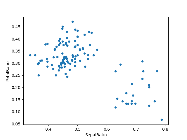
由于传入了一个函数,因此该函数是在分配给的DataFrame上计算的。重要的是,这是经过过滤的DataFrame,它被过滤到那些花冠长度大于5的行。首先进行过滤,然后计算比率。这是一个我们没有引用 滤过 提供DataFrame。
的函数签名 assign() 就是简单地 **kwargs 。键是新字段的列名,值是要插入的值(例如 Series 或NumPy数组),或要在 DataFrame 。一个 copy 原作的 DataFrame 返回,并插入新值。
的顺序 **kwargs 被保存了下来。这允许 依赖于 赋值,其中后面的表达式 **kwargs 中创建的列可以引用 assign() 。
In [90]: dfa = pd.DataFrame({"A": [1, 2, 3], "B": [4, 5, 6]})

In [91]: dfa.assign(C=lambda x: x["A"] + x["B"], D=lambda x: x["A"] + x["C"])
Out[91]:
   A  B  C   D
0  1  4  5   6
1  2  5  7   9
2  3  6  9  12
在第二个表达式中, x['C'] 将引用新创建的列,这等于 dfa['A'] + dfa['B'] 。
索引/选择#
索引的基本知识如下:
运营 |
语法 |
结果 |
|---|---|---|
选择列 |
|
系列 |
按标签选择行 |
|
系列 |
按整数位置选择行 |
|
系列 |
对行进行切片 |
|
DataFrame |
按布尔向量选择行 |
|
DataFrame |
例如,行选择返回一个 Series 其索引是 DataFrame :
In [92]: df.loc["b"]
Out[92]:
one            2.0
bar            2.0
flag         False
foo            bar
one_trunc      2.0
Name: b, dtype: object

In [93]: df.iloc[2]
Out[93]:
one           3.0
bar           3.0
flag         True
foo           bar
one_trunc     NaN
Name: c, dtype: object
有关复杂的基于标签的索引和切片的更详尽的处理,请参阅 section on indexing 。我们将在中介绍重新编制索引/符合新标签集的基本原理 section on reindexing 。
数据对齐和算法#
之间的数据对齐 DataFrame 对象自动对齐打开 列和索引(行标签) 。同样,得到的对象将具有列标签和行标签的并集。
In [94]: df = pd.DataFrame(np.random.randn(10, 4), columns=["A", "B", "C", "D"])

In [95]: df2 = pd.DataFrame(np.random.randn(7, 3), columns=["A", "B", "C"])

In [96]: df + df2
Out[96]:
          A         B         C   D
0  0.045691 -0.014138  1.380871 NaN
1 -0.955398 -1.501007  0.037181 NaN
2 -0.662690  1.534833 -0.859691 NaN
3 -2.452949  1.237274 -0.133712 NaN
4  1.414490  1.951676 -2.320422 NaN
5 -0.494922 -1.649727 -1.084601 NaN
6 -1.047551 -0.748572 -0.805479 NaN
7       NaN       NaN       NaN NaN
8       NaN       NaN       NaN NaN
9       NaN       NaN       NaN NaN
When doing an operation between DataFrame and Series, the default behavior is
to align the Series index on the DataFrame columns, thus broadcasting
row-wise. For example:
In [97]: df - df.iloc[0]
Out[97]:
          A         B         C         D
0  0.000000  0.000000  0.000000  0.000000
1 -1.359261 -0.248717 -0.453372 -1.754659
2  0.253128  0.829678  0.010026 -1.991234
3 -1.311128  0.054325 -1.724913 -1.620544
4  0.573025  1.500742 -0.676070  1.367331
5 -1.741248  0.781993 -1.241620 -2.053136
6 -1.240774 -0.869551 -0.153282  0.000430
7 -0.743894  0.411013 -0.929563 -0.282386
8 -1.194921  1.320690  0.238224 -1.482644
9  2.293786  1.856228  0.773289 -1.446531
有关对匹配和广播行为的显式控制,请参阅 flexible binary operations 。
使用标量的算术运算按元素操作:
In [98]: df * 5 + 2
Out[98]:
           A         B         C          D
0   3.359299 -0.124862  4.835102   3.381160
1  -3.437003 -1.368449  2.568242  -5.392133
2   4.624938  4.023526  4.885230  -6.575010
3  -3.196342  0.146766 -3.789461  -4.721559
4   6.224426  7.378849  1.454750  10.217815
5  -5.346940  3.785103 -1.373001  -6.884519
6  -2.844569 -4.472618  4.068691   3.383309
7  -0.360173  1.930201  0.187285   1.969232
8  -2.615303  6.478587  6.026220  -4.032059
9  14.828230  9.156280  8.701544  -3.851494

In [99]: 1 / df
Out[99]:
          A          B         C           D
0  3.678365  -2.353094  1.763605    3.620145
1 -0.919624  -1.484363  8.799067   -0.676395
2  1.904807   2.470934  1.732964   -0.583090
3 -0.962215  -2.697986 -0.863638   -0.743875
4  1.183593   0.929567 -9.170108    0.608434
5 -0.680555   2.800959 -1.482360   -0.562777
6 -1.032084  -0.772485  2.416988    3.614523
7 -2.118489 -71.634509 -2.758294 -162.507295
8 -1.083352   1.116424  1.241860   -0.828904
9  0.389765   0.698687  0.746097   -0.854483

In [100]: df ** 4
Out[100]:
           A             B         C             D
0   0.005462  3.261689e-02  0.103370  5.822320e-03
1   1.398165  2.059869e-01  0.000167  4.777482e+00
2   0.075962  2.682596e-02  0.110877  8.650845e+00
3   1.166571  1.887302e-02  1.797515  3.265879e+00
4   0.509555  1.339298e+00  0.000141  7.297019e+00
5   4.661717  1.624699e-02  0.207103  9.969092e+00
6   0.881334  2.808277e+00  0.029302  5.858632e-03
7   0.049647  3.797614e-08  0.017276  1.433866e-09
8   0.725974  6.437005e-01  0.420446  2.118275e+00
9  43.329821  4.196326e+00  3.227153  1.875802e+00
布尔运算符也按元素操作:
In [101]: df1 = pd.DataFrame({"a": [1, 0, 1], "b": [0, 1, 1]}, dtype=bool)

In [102]: df2 = pd.DataFrame({"a": [0, 1, 1], "b": [1, 1, 0]}, dtype=bool)

In [103]: df1 & df2
Out[103]:
       a      b
0  False  False
1  False   True
2   True  False

In [104]: df1 | df2
Out[104]:
      a     b
0  True  True
1  True  True
2  True  True

In [105]: df1 ^ df2
Out[105]:
       a      b
0   True   True
1   True  False
2  False   True

In [106]: -df1
Out[106]:
       a      b
0  False   True
1   True  False
2  False  False
换位#
若要转置,请访问 T 属性或 DataFrame.transpose() ,类似于ndarray:
# only show the first 5 rows
In [107]: df[:5].T
Out[107]:
          0         1         2         3         4
A  0.271860 -1.087401  0.524988 -1.039268  0.844885
B -0.424972 -0.673690  0.404705 -0.370647  1.075770
C  0.567020  0.113648  0.577046 -1.157892 -0.109050
D  0.276232 -1.478427 -1.715002 -1.344312  1.643563
DataFrame与NumPy函数的互操作性#
大多数NumPy函数都可以直接在 Series 和 DataFrame 。
In [108]: np.exp(df)
Out[108]:
           A         B         C         D
0   1.312403  0.653788  1.763006  1.318154
1   0.337092  0.509824  1.120358  0.227996
2   1.690438  1.498861  1.780770  0.179963
3   0.353713  0.690288  0.314148  0.260719
4   2.327710  2.932249  0.896686  5.173571
5   0.230066  1.429065  0.509360  0.169161
6   0.379495  0.274028  1.512461  1.318720
7   0.623732  0.986137  0.695904  0.993865
8   0.397301  2.449092  2.237242  0.299269
9  13.009059  4.183951  3.820223  0.310274

In [109]: np.asarray(df)
Out[109]:
array([[ 0.2719, -0.425 ,  0.567 ,  0.2762],
       [-1.0874, -0.6737,  0.1136, -1.4784],
       [ 0.525 ,  0.4047,  0.577 , -1.715 ],
       [-1.0393, -0.3706, -1.1579, -1.3443],
       [ 0.8449,  1.0758, -0.109 ,  1.6436],
       [-1.4694,  0.357 , -0.6746, -1.7769],
       [-0.9689, -1.2945,  0.4137,  0.2767],
       [-0.472 , -0.014 , -0.3625, -0.0062],
       [-0.9231,  0.8957,  0.8052, -1.2064],
       [ 2.5656,  1.4313,  1.3403, -1.1703]])
DataFrame 并不打算替代ndarray,因为它的索引语义和数据模型在某些地方与n维数组有很大不同。
Series 机具 __array_ufunc__ ,这使得它可以与NumPy的 universal functions 。
Ufunc应用于基础数组的 Series 。
In [110]: ser = pd.Series([1, 2, 3, 4])

In [111]: np.exp(ser)
Out[111]:
0     2.718282
1     7.389056
2    20.085537
3    54.598150
dtype: float64
在 0.25.0 版更改: 当多个 Series 传递给ufunc,则在执行操作之前对齐它们。
像类库的其他部分一样,Pandas将自动将标记的输入与多个输入对齐,作为ufunc的一部分。例如,使用 numpy.remainder() 数到两 Series 具有不同排序的标签将在操作前对齐。
In [112]: ser1 = pd.Series([1, 2, 3], index=["a", "b", "c"])

In [113]: ser2 = pd.Series([1, 3, 5], index=["b", "a", "c"])

In [114]: ser1
Out[114]:
a    1
b    2
c    3
dtype: int64

In [115]: ser2
Out[115]:
b    1
a    3
c    5
dtype: int64

In [116]: np.remainder(ser1, ser2)
Out[116]:
a    1
b    0
c    3
dtype: int64
像往常一样,取两个索引的并集,不重叠的值用缺失值填充。
In [117]: ser3 = pd.Series([2, 4, 6], index=["b", "c", "d"])

In [118]: ser3
Out[118]:
b    2
c    4
d    6
dtype: int64

In [119]: np.remainder(ser1, ser3)
Out[119]:
a    NaN
b    0.0
c    3.0
d    NaN
dtype: float64
当二进制ufunc应用于 Series 和 Index ,即 Series 实现优先,并且 Series 返回。
In [120]: ser = pd.Series([1, 2, 3])

In [121]: idx = pd.Index([4, 5, 6])

In [122]: np.maximum(ser, idx)
Out[122]:
0    4
1    5
2    6
dtype: int64
可以安全地应用NumPy uuncs Series 例如,由非ndarray阵列支持 arrays.SparseArray (请参阅 稀疏计算 )。如果可能,在不将底层数据转换为ndarray的情况下应用ufunc。
控制台显示#
一个非常大的 DataFrame 将被截断以在控制台中显示它们。您还可以使用以下命令获取摘要 info() 。( 棒球 数据集来自 plyr R包):
In [123]: baseball = pd.read_csv("data/baseball.csv")

In [124]: print(baseball)
       id     player  year  stint team  lg   g   ab   r    h  X2b  X3b  hr   rbi   sb   cs  bb    so  ibb  hbp   sh   sf  gidp
0   88641  womacto01  2006      2  CHN  NL  19   50   6   14    1    0   1   2.0  1.0  1.0   4   4.0  0.0  0.0  3.0  0.0   0.0
1   88643  schilcu01  2006      1  BOS  AL  31    2   0    1    0    0   0   0.0  0.0  0.0   0   1.0  0.0  0.0  0.0  0.0   0.0
..    ...        ...   ...    ...  ...  ..  ..  ...  ..  ...  ...  ...  ..   ...  ...  ...  ..   ...  ...  ...  ...  ...   ...
98  89533   aloumo01  2007      1  NYN  NL  87  328  51  112   19    1  13  49.0  3.0  0.0  27  30.0  5.0  2.0  0.0  3.0  13.0
99  89534  alomasa02  2007      1  NYN  NL   8   22   1    3    1    0   0   0.0  0.0  0.0   0   3.0  0.0  0.0  0.0  0.0   0.0

[100 rows x 23 columns]

In [125]: baseball.info()
<class 'pandas.core.frame.DataFrame'>
RangeIndex: 100 entries, 0 to 99
Data columns (total 23 columns):
 #   Column  Non-Null Count  Dtype
---  ------  --------------  -----
 0   id      100 non-null    int64
 1   player  100 non-null    object
 2   year    100 non-null    int64
 3   stint   100 non-null    int64
 4   team    100 non-null    object
 5   lg      100 non-null    object
 6   g       100 non-null    int64
 7   ab      100 non-null    int64
 8   r       100 non-null    int64
 9   h       100 non-null    int64
 10  X2b     100 non-null    int64
 11  X3b     100 non-null    int64
 12  hr      100 non-null    int64
 13  rbi     100 non-null    float64
 14  sb      100 non-null    float64
 15  cs      100 non-null    float64
 16  bb      100 non-null    int64
 17  so      100 non-null    float64
 18  ibb     100 non-null    float64
 19  hbp     100 non-null    float64
 20  sh      100 non-null    float64
 21  sf      100 non-null    float64
 22  gidp    100 non-null    float64
dtypes: float64(9), int64(11), object(3)
memory usage: 18.1+ KB
但是,使用 DataFrame.to_string() 将返回 DataFrame 表格形式,尽管它并不总是适合控制台宽度:
In [126]: print(baseball.iloc[-20:, :12].to_string())
       id     player  year  stint team  lg    g   ab   r    h  X2b  X3b
80  89474  finlest01  2007      1  COL  NL   43   94   9   17    3    0
81  89480  embreal01  2007      1  OAK  AL    4    0   0    0    0    0
82  89481  edmonji01  2007      1  SLN  NL  117  365  39   92   15    2
83  89482  easleda01  2007      1  NYN  NL   76  193  24   54    6    0
84  89489  delgaca01  2007      1  NYN  NL  139  538  71  139   30    0
85  89493  cormirh01  2007      1  CIN  NL    6    0   0    0    0    0
86  89494  coninje01  2007      2  NYN  NL   21   41   2    8    2    0
87  89495  coninje01  2007      1  CIN  NL   80  215  23   57   11    1
88  89497  clemero02  2007      1  NYA  AL    2    2   0    1    0    0
89  89498  claytro01  2007      2  BOS  AL    8    6   1    0    0    0
90  89499  claytro01  2007      1  TOR  AL   69  189  23   48   14    0
91  89501  cirilje01  2007      2  ARI  NL   28   40   6    8    4    0
92  89502  cirilje01  2007      1  MIN  AL   50  153  18   40    9    2
93  89521  bondsba01  2007      1  SFN  NL  126  340  75   94   14    0
94  89523  biggicr01  2007      1  HOU  NL  141  517  68  130   31    3
95  89525  benitar01  2007      2  FLO  NL   34    0   0    0    0    0
96  89526  benitar01  2007      1  SFN  NL   19    0   0    0    0    0
97  89530  ausmubr01  2007      1  HOU  NL  117  349  38   82   16    3
98  89533   aloumo01  2007      1  NYN  NL   87  328  51  112   19    1
99  89534  alomasa02  2007      1  NYN  NL    8   22   1    3    1    0
默认情况下,宽数据帧将跨多行打印:
In [127]: pd.DataFrame(np.random.randn(3, 12))
Out[127]:
         0         1         2         3         4         5         6         7         8         9         10        11
0 -1.226825  0.769804 -1.281247 -0.727707 -0.121306 -0.097883  0.695775  0.341734  0.959726 -1.110336 -0.619976  0.149748
1 -0.732339  0.687738  0.176444  0.403310 -0.154951  0.301624 -2.179861 -1.369849 -0.954208  1.462696 -1.743161 -0.826591
2 -0.345352  1.314232  0.690579  0.995761  2.396780  0.014871  3.357427 -0.317441 -1.236269  0.896171 -0.487602 -0.082240
属性可以更改单行上的打印量。 display.width 选项:
In [128]: pd.set_option("display.width", 40)  # default is 80

In [129]: pd.DataFrame(np.random.randn(3, 12))
Out[129]:
         0         1         2         3         4         5         6         7         8         9         10        11
0 -2.182937  0.380396  0.084844  0.432390  1.519970 -0.493662  0.600178  0.274230  0.132885 -0.023688  2.410179  1.450520
1  0.206053 -0.251905 -2.213588  1.063327  1.266143  0.299368 -0.863838  0.408204 -1.048089 -0.025747 -0.988387  0.094055
2  1.262731  1.289997  0.082423 -0.055758  0.536580 -0.489682  0.369374 -0.034571 -2.484478 -0.281461  0.030711  0.109121
可以通过设置来调整各个列的最大宽度 display.max_colwidth
In [130]: datafile = {
   .....:     "filename": ["filename_01", "filename_02"],
   .....:     "path": [
   .....:         "media/user_name/storage/folder_01/filename_01",
   .....:         "media/user_name/storage/folder_02/filename_02",
   .....:     ],
   .....: }
   .....:

In [131]: pd.set_option("display.max_colwidth", 30)

In [132]: pd.DataFrame(datafile)
Out[132]:
      filename                           path
0  filename_01  media/user_name/storage/fo...
1  filename_02  media/user_name/storage/fo...

In [133]: pd.set_option("display.max_colwidth", 100)

In [134]: pd.DataFrame(datafile)
Out[134]:
      filename                                           path
0  filename_01  media/user_name/storage/folder_01/filename_01
1  filename_02  media/user_name/storage/folder_02/filename_02
您也可以通过以下方式禁用此功能 expand_frame_repr 选择。这将在一个块中打印表。
DataFrame列属性访问和IPython完成#
如果一个 DataFrame Column Label是有效的Python变量名,可以像属性一样访问该列:
In [135]: df = pd.DataFrame({"foo1": np.random.randn(5), "foo2": np.random.randn(5)})

In [136]: df
Out[136]:
       foo1      foo2
0  1.126203  0.781836
1 -0.977349 -1.071357
2  1.474071  0.441153
3 -0.064034  2.353925
4 -1.282782  0.583787

In [137]: df.foo1
Out[137]:
0    1.126203
1   -0.977349
2    1.474071
3   -0.064034
4   -1.282782
Name: foo1, dtype: float64
这些柱还连接到 IPython 完成机制,以便它们可以按Tab键完成:
In [5]: df.foo<TAB>  # noqa: E225, E999
df.foo1  df.foo2