烹饪书#
这是一个存储库 短小精悍 有用的Pandas食谱的例子和链接。我们鼓励用户在此文档中添加内容。
在这一部分添加有趣的链接和/或内联示例是一个很好的选择 第一个拉取请求 。
在可能的地方插入了简化的、精简的、对新用户友好的内联示例,以增强Stack-Overflow和GitHub链接。在内联示例提供的内容之上,许多链接都包含扩展信息。
Pandas(Pd)和NumPy(NP)是仅有的两个缩写的进口模块。其余的则为新用户保留显式导入。
成语#
这些是一些整洁的Pandas idioms
if-then/if-then-else on one column, and assignment to another one or more columns:
In [1]: df = pd.DataFrame(
   ...:     {"AAA": [4, 5, 6, 7], "BBB": [10, 20, 30, 40], "CCC": [100, 50, -30, -50]}
   ...: )
   ...:

In [2]: df
Out[2]:
   AAA  BBB  CCC
0    4   10  100
1    5   20   50
2    6   30  -30
3    7   40  -50
如果-那么.#
一列上的If-Then
In [3]: df.loc[df.AAA >= 5, "BBB"] = -1

In [4]: df
Out[4]:
   AAA  BBB  CCC
0    4   10  100
1    5   -1   50
2    6   -1  -30
3    7   -1  -50
分配给2列的IF-THEN:
In [5]: df.loc[df.AAA >= 5, ["BBB", "CCC"]] = 555

In [6]: df
Out[6]:
   AAA  BBB  CCC
0    4   10  100
1    5  555  555
2    6  555  555
3    7  555  555
添加具有不同逻辑的另一行,以执行-Else
In [7]: df.loc[df.AAA < 5, ["BBB", "CCC"]] = 2000

In [8]: df
Out[8]:
   AAA   BBB   CCC
0    4  2000  2000
1    5   555   555
2    6   555   555
3    7   555   555
或者在你戴好面具后用Pandas
In [9]: df_mask = pd.DataFrame(
   ...:     {"AAA": [True] * 4, "BBB": [False] * 4, "CCC": [True, False] * 2}
   ...: )
   ...:

In [10]: df.where(df_mask, -1000)
Out[10]:
   AAA   BBB   CCC
0    4 -1000  2000
1    5 -1000 -1000
2    6 -1000   555
3    7 -1000 -1000
if-then-else using NumPy's where()
In [11]: df = pd.DataFrame(
   ....:     {"AAA": [4, 5, 6, 7], "BBB": [10, 20, 30, 40], "CCC": [100, 50, -30, -50]}
   ....: )
   ....:

In [12]: df
Out[12]:
   AAA  BBB  CCC
0    4   10  100
1    5   20   50
2    6   30  -30
3    7   40  -50

In [13]: df["logic"] = np.where(df["AAA"] > 5, "high", "low")

In [14]: df
Out[14]:
   AAA  BBB  CCC logic
0    4   10  100   low
1    5   20   50   low
2    6   30  -30  high
3    7   40  -50  high
拆分#
Split a frame with a boolean criterion
In [15]: df = pd.DataFrame(
   ....:     {"AAA": [4, 5, 6, 7], "BBB": [10, 20, 30, 40], "CCC": [100, 50, -30, -50]}
   ....: )
   ....:

In [16]: df
Out[16]:
   AAA  BBB  CCC
0    4   10  100
1    5   20   50
2    6   30  -30
3    7   40  -50

In [17]: df[df.AAA <= 5]
Out[17]:
   AAA  BBB  CCC
0    4   10  100
1    5   20   50

In [18]: df[df.AAA > 5]
Out[18]:
   AAA  BBB  CCC
2    6   30  -30
3    7   40  -50
建筑标准#
Select with multi-column criteria
In [19]: df = pd.DataFrame(
   ....:     {"AAA": [4, 5, 6, 7], "BBB": [10, 20, 30, 40], "CCC": [100, 50, -30, -50]}
   ....: )
   ....:

In [20]: df
Out[20]:
   AAA  BBB  CCC
0    4   10  100
1    5   20   50
2    6   30  -30
3    7   40  -50
...AND(未赋值时返回一个系列)
In [21]: df.loc[(df["BBB"] < 25) & (df["CCC"] >= -40), "AAA"]
Out[21]:
0    4
1    5
Name: AAA, dtype: int64
...或(未赋值时返回一个系列)
In [22]: df.loc[(df["BBB"] > 25) | (df["CCC"] >= -40), "AAA"]
Out[22]:
0    4
1    5
2    6
3    7
Name: AAA, dtype: int64
...或(使用赋值来修改DataFrame。)
In [23]: df.loc[(df["BBB"] > 25) | (df["CCC"] >= 75), "AAA"] = 0.1

In [24]: df
Out[24]:
   AAA  BBB  CCC
0  0.1   10  100
1  5.0   20   50
2  0.1   30  -30
3  0.1   40  -50
Select rows with data closest to certain value using argsort
In [25]: df = pd.DataFrame(
   ....:     {"AAA": [4, 5, 6, 7], "BBB": [10, 20, 30, 40], "CCC": [100, 50, -30, -50]}
   ....: )
   ....:

In [26]: df
Out[26]:
   AAA  BBB  CCC
0    4   10  100
1    5   20   50
2    6   30  -30
3    7   40  -50

In [27]: aValue = 43.0

In [28]: df.loc[(df.CCC - aValue).abs().argsort()]
Out[28]:
   AAA  BBB  CCC
1    5   20   50
0    4   10  100
2    6   30  -30
3    7   40  -50
Dynamically reduce a list of criteria using a binary operators
In [29]: df = pd.DataFrame(
   ....:     {"AAA": [4, 5, 6, 7], "BBB": [10, 20, 30, 40], "CCC": [100, 50, -30, -50]}
   ....: )
   ....:

In [30]: df
Out[30]:
   AAA  BBB  CCC
0    4   10  100
1    5   20   50
2    6   30  -30
3    7   40  -50

In [31]: Crit1 = df.AAA <= 5.5

In [32]: Crit2 = df.BBB == 10.0

In [33]: Crit3 = df.CCC > -40.0
人们可以硬编码:
In [34]: AllCrit = Crit1 & Crit2 & Crit3
...或者可以使用动态构建的标准列表来完成
In [35]: import functools

In [36]: CritList = [Crit1, Crit2, Crit3]

In [37]: AllCrit = functools.reduce(lambda x, y: x & y, CritList)

In [38]: df[AllCrit]
Out[38]:
   AAA  BBB  CCC
0    4   10  100
选择#
数据帧#
这个 indexing 医生。
Using both row labels and value conditionals
In [39]: df = pd.DataFrame(
   ....:     {"AAA": [4, 5, 6, 7], "BBB": [10, 20, 30, 40], "CCC": [100, 50, -30, -50]}
   ....: )
   ....:

In [40]: df
Out[40]:
   AAA  BBB  CCC
0    4   10  100
1    5   20   50
2    6   30  -30
3    7   40  -50

In [41]: df[(df.AAA <= 6) & (df.index.isin([0, 2, 4]))]
Out[41]:
   AAA  BBB  CCC
0    4   10  100
2    6   30  -30
使用loc进行面向标签的切片和iloc位置切片 GH2904
In [42]: df = pd.DataFrame(
   ....:     {"AAA": [4, 5, 6, 7], "BBB": [10, 20, 30, 40], "CCC": [100, 50, -30, -50]},
   ....:     index=["foo", "bar", "boo", "kar"],
   ....: )
   ....:
有两种显式切片方法,还有第三种一般情况
面向位置(Python切片样式:不包括END)
面向标签(非Python切片样式:包括END)
常规(切片样式:取决于切片是否包含标签或位置)
In [43]: df.loc["bar":"kar"]  # Label
Out[43]:
     AAA  BBB  CCC
bar    5   20   50
boo    6   30  -30
kar    7   40  -50

# Generic
In [44]: df[0:3]
Out[44]:
     AAA  BBB  CCC
foo    4   10  100
bar    5   20   50
boo    6   30  -30

In [45]: df["bar":"kar"]
Out[45]:
     AAA  BBB  CCC
bar    5   20   50
boo    6   30  -30
kar    7   40  -50
当索引由非零开始或非单位增量的整数组成时,就会出现歧义。
In [46]: data = {"AAA": [4, 5, 6, 7], "BBB": [10, 20, 30, 40], "CCC": [100, 50, -30, -50]}

In [47]: df2 = pd.DataFrame(data=data, index=[1, 2, 3, 4])  # Note index starts at 1.

In [48]: df2.iloc[1:3]  # Position-oriented
Out[48]:
   AAA  BBB  CCC
2    5   20   50
3    6   30  -30

In [49]: df2.loc[1:3]  # Label-oriented
Out[49]:
   AAA  BBB  CCC
1    4   10  100
2    5   20   50
3    6   30  -30
Using inverse operator (~) to take the complement of a mask
In [50]: df = pd.DataFrame(
   ....:     {"AAA": [4, 5, 6, 7], "BBB": [10, 20, 30, 40], "CCC": [100, 50, -30, -50]}
   ....: )
   ....:

In [51]: df
Out[51]:
   AAA  BBB  CCC
0    4   10  100
1    5   20   50
2    6   30  -30
3    7   40  -50

In [52]: df[~((df.AAA <= 6) & (df.index.isin([0, 2, 4])))]
Out[52]:
   AAA  BBB  CCC
1    5   20   50
3    7   40  -50
新列#
Efficiently and dynamically creating new columns using applymap
In [53]: df = pd.DataFrame({"AAA": [1, 2, 1, 3], "BBB": [1, 1, 2, 2], "CCC": [2, 1, 3, 1]})

In [54]: df
Out[54]:
   AAA  BBB  CCC
0    1    1    2
1    2    1    1
2    1    2    3
3    3    2    1

In [55]: source_cols = df.columns  # Or some subset would work too

In [56]: new_cols = [str(x) + "_cat" for x in source_cols]

In [57]: categories = {1: "Alpha", 2: "Beta", 3: "Charlie"}

In [58]: df[new_cols] = df[source_cols].applymap(categories.get)

In [59]: df
Out[59]:
   AAA  BBB  CCC  AAA_cat BBB_cat  CCC_cat
0    1    1    2    Alpha   Alpha     Beta
1    2    1    1     Beta   Alpha    Alpha
2    1    2    3    Alpha    Beta  Charlie
3    3    2    1  Charlie    Beta    Alpha
Keep other columns when using min() with groupby
In [60]: df = pd.DataFrame(
   ....:     {"AAA": [1, 1, 1, 2, 2, 2, 3, 3], "BBB": [2, 1, 3, 4, 5, 1, 2, 3]}
   ....: )
   ....:

In [61]: df
Out[61]:
   AAA  BBB
0    1    2
1    1    1
2    1    3
3    2    4
4    2    5
5    2    1
6    3    2
7    3    3
方法1:idxmin()获取最小值的索引
In [62]: df.loc[df.groupby("AAA")["BBB"].idxmin()]
Out[62]:
   AAA  BBB
1    1    1
5    2    1
6    3    2
方法2:先排序,然后取第一个
In [63]: df.sort_values(by="BBB").groupby("AAA", as_index=False).first()
Out[63]:
   AAA  BBB
0    1    1
1    2    1
2    3    2
请注意相同的结果,但索引除外。
多索引#
这个 multindexing 医生。
Creating a MultiIndex from a labeled frame
In [64]: df = pd.DataFrame(
   ....:     {
   ....:         "row": [0, 1, 2],
   ....:         "One_X": [1.1, 1.1, 1.1],
   ....:         "One_Y": [1.2, 1.2, 1.2],
   ....:         "Two_X": [1.11, 1.11, 1.11],
   ....:         "Two_Y": [1.22, 1.22, 1.22],
   ....:     }
   ....: )
   ....:

In [65]: df
Out[65]:
   row  One_X  One_Y  Two_X  Two_Y
0    0    1.1    1.2   1.11   1.22
1    1    1.1    1.2   1.11   1.22
2    2    1.1    1.2   1.11   1.22

# As Labelled Index
In [66]: df = df.set_index("row")

In [67]: df
Out[67]:
     One_X  One_Y  Two_X  Two_Y
row
0      1.1    1.2   1.11   1.22
1      1.1    1.2   1.11   1.22
2      1.1    1.2   1.11   1.22

# With Hierarchical Columns
In [68]: df.columns = pd.MultiIndex.from_tuples([tuple(c.split("_")) for c in df.columns])

In [69]: df
Out[69]:
     One        Two
       X    Y     X     Y
row
0    1.1  1.2  1.11  1.22
1    1.1  1.2  1.11  1.22
2    1.1  1.2  1.11  1.22

# Now stack & Reset
In [70]: df = df.stack(0).reset_index(1)

In [71]: df
Out[71]:
    level_1     X     Y
row
0       One  1.10  1.20
0       Two  1.11  1.22
1       One  1.10  1.20
1       Two  1.11  1.22
2       One  1.10  1.20
2       Two  1.11  1.22

# And fix the labels (Notice the label 'level_1' got added automatically)
In [72]: df.columns = ["Sample", "All_X", "All_Y"]

In [73]: df
Out[73]:
    Sample  All_X  All_Y
row
0      One   1.10   1.20
0      Two   1.11   1.22
1      One   1.10   1.20
1      Two   1.11   1.22
2      One   1.10   1.20
2      Two   1.11   1.22
算术#
Performing arithmetic with a MultiIndex that needs broadcasting
In [74]: cols = pd.MultiIndex.from_tuples(
   ....:     [(x, y) for x in ["A", "B", "C"] for y in ["O", "I"]]
   ....: )
   ....:

In [75]: df = pd.DataFrame(np.random.randn(2, 6), index=["n", "m"], columns=cols)

In [76]: df
Out[76]:
          A                   B                   C
          O         I         O         I         O         I
n  0.469112 -0.282863 -1.509059 -1.135632  1.212112 -0.173215
m  0.119209 -1.044236 -0.861849 -2.104569 -0.494929  1.071804

In [77]: df = df.div(df["C"], level=1)

In [78]: df
Out[78]:
          A                   B              C
          O         I         O         I    O    I
n  0.387021  1.633022 -1.244983  6.556214  1.0  1.0
m -0.240860 -0.974279  1.741358 -1.963577  1.0  1.0
切片#
In [79]: coords = [("AA", "one"), ("AA", "six"), ("BB", "one"), ("BB", "two"), ("BB", "six")]

In [80]: index = pd.MultiIndex.from_tuples(coords)

In [81]: df = pd.DataFrame([11, 22, 33, 44, 55], index, ["MyData"])

In [82]: df
Out[82]:
        MyData
AA one      11
   six      22
BB one      33
   two      44
   six      55
要获取第1层和第1轴的横截面,请执行以下操作:
# Note : level and axis are optional, and default to zero
In [83]: df.xs("BB", level=0, axis=0)
Out[83]:
     MyData
one      33
two      44
six      55
...现在是第一轴的第二层。
In [84]: df.xs("six", level=1, axis=0)
Out[84]:
    MyData
AA      22
BB      55
Slicing a MultiIndex with xs, method #2
In [85]: import itertools

In [86]: index = list(itertools.product(["Ada", "Quinn", "Violet"], ["Comp", "Math", "Sci"]))

In [87]: headr = list(itertools.product(["Exams", "Labs"], ["I", "II"]))

In [88]: indx = pd.MultiIndex.from_tuples(index, names=["Student", "Course"])

In [89]: cols = pd.MultiIndex.from_tuples(headr)  # Notice these are un-named

In [90]: data = [[70 + x + y + (x * y) % 3 for x in range(4)] for y in range(9)]

In [91]: df = pd.DataFrame(data, indx, cols)

In [92]: df
Out[92]:
               Exams     Labs
                   I  II    I  II
Student Course
Ada     Comp      70  71   72  73
        Math      71  73   75  74
        Sci       72  75   75  75
Quinn   Comp      73  74   75  76
        Math      74  76   78  77
        Sci       75  78   78  78
Violet  Comp      76  77   78  79
        Math      77  79   81  80
        Sci       78  81   81  81

In [93]: All = slice(None)

In [94]: df.loc["Violet"]
Out[94]:
       Exams     Labs
           I  II    I  II
Course
Comp      76  77   78  79
Math      77  79   81  80
Sci       78  81   81  81

In [95]: df.loc[(All, "Math"), All]
Out[95]:
               Exams     Labs
                   I  II    I  II
Student Course
Ada     Math      71  73   75  74
Quinn   Math      74  76   78  77
Violet  Math      77  79   81  80

In [96]: df.loc[(slice("Ada", "Quinn"), "Math"), All]
Out[96]:
               Exams     Labs
                   I  II    I  II
Student Course
Ada     Math      71  73   75  74
Quinn   Math      74  76   78  77

In [97]: df.loc[(All, "Math"), ("Exams")]
Out[97]:
                 I  II
Student Course
Ada     Math    71  73
Quinn   Math    74  76
Violet  Math    77  79

In [98]: df.loc[(All, "Math"), (All, "II")]
Out[98]:
               Exams Labs
                  II   II
Student Course
Ada     Math      73   74
Quinn   Math      76   77
Violet  Math      79   80
分选#
Sort by specific column or an ordered list of columns, with a MultiIndex
In [99]: df.sort_values(by=("Labs", "II"), ascending=False)
Out[99]:
               Exams     Labs
                   I  II    I  II
Student Course
Violet  Sci       78  81   81  81
        Math      77  79   81  80
        Comp      76  77   78  79
Quinn   Sci       75  78   78  78
        Math      74  76   78  77
        Comp      73  74   75  76
Ada     Sci       72  75   75  75
        Math      71  73   75  74
        Comp      70  71   72  73
部分选择,分类的需要 GH2995
级别#
缺少数据#
这个 missing data 医生。
向前填充一个倒转的时间序列
In [100]: df = pd.DataFrame(
   .....:     np.random.randn(6, 1),
   .....:     index=pd.date_range("2013-08-01", periods=6, freq="B"),
   .....:     columns=list("A"),
   .....: )
   .....:

In [101]: df.loc[df.index[3], "A"] = np.nan

In [102]: df
Out[102]:
                   A
2013-08-01  0.721555
2013-08-02 -0.706771
2013-08-05 -1.039575
2013-08-06       NaN
2013-08-07 -0.424972
2013-08-08  0.567020

In [103]: df.bfill()
Out[103]:
                   A
2013-08-01  0.721555
2013-08-02 -0.706771
2013-08-05 -1.039575
2013-08-06 -0.424972
2013-08-07 -0.424972
2013-08-08  0.567020
替换#
分组#
这个 grouping 医生。
与agg不同,Apply的Callable被传递给一个子DataFrame,它允许您访问所有列
In [104]: df = pd.DataFrame(
   .....:     {
   .....:         "animal": "cat dog cat fish dog cat cat".split(),
   .....:         "size": list("SSMMMLL"),
   .....:         "weight": [8, 10, 11, 1, 20, 12, 12],
   .....:         "adult": [False] * 5 + [True] * 2,
   .....:     }
   .....: )
   .....:

In [105]: df
Out[105]:
  animal size  weight  adult
0    cat    S       8  False
1    dog    S      10  False
2    cat    M      11  False
3   fish    M       1  False
4    dog    M      20  False
5    cat    L      12   True
6    cat    L      12   True

# List the size of the animals with the highest weight.
In [106]: df.groupby("animal").apply(lambda subf: subf["size"][subf["weight"].idxmax()])
Out[106]:
animal
cat     L
dog     M
fish    M
dtype: object
In [107]: gb = df.groupby(["animal"])

In [108]: gb.get_group("cat")
Out[108]:
  animal size  weight  adult
0    cat    S       8  False
2    cat    M      11  False
5    cat    L      12   True
6    cat    L      12   True
Apply to different items in a group
In [109]: def GrowUp(x):
   .....:     avg_weight = sum(x[x["size"] == "S"].weight * 1.5)
   .....:     avg_weight += sum(x[x["size"] == "M"].weight * 1.25)
   .....:     avg_weight += sum(x[x["size"] == "L"].weight)
   .....:     avg_weight /= len(x)
   .....:     return pd.Series(["L", avg_weight, True], index=["size", "weight", "adult"])
   .....:

In [110]: expected_df = gb.apply(GrowUp)

In [111]: expected_df
Out[111]:
       size   weight  adult
animal
cat       L  12.4375   True
dog       L  20.0000   True
fish      L   1.2500   True
In [112]: S = pd.Series([i / 100.0 for i in range(1, 11)])

In [113]: def cum_ret(x, y):
   .....:     return x * (1 + y)
   .....:

In [114]: def red(x):
   .....:     return functools.reduce(cum_ret, x, 1.0)
   .....:

In [115]: S.expanding().apply(red, raw=True)
Out[115]:
0    1.010000
1    1.030200
2    1.061106
3    1.103550
4    1.158728
5    1.228251
6    1.314229
7    1.419367
8    1.547110
9    1.701821
dtype: float64
Replacing some values with mean of the rest of a group
In [116]: df = pd.DataFrame({"A": [1, 1, 2, 2], "B": [1, -1, 1, 2]})

In [117]: gb = df.groupby("A")

In [118]: def replace(g):
   .....:     mask = g < 0
   .....:     return g.where(mask, g[~mask].mean())
   .....:

In [119]: gb.transform(replace)
Out[119]:
     B
0  1.0
1 -1.0
2  1.5
3  1.5
Sort groups by aggregated data
In [120]: df = pd.DataFrame(
   .....:     {
   .....:         "code": ["foo", "bar", "baz"] * 2,
   .....:         "data": [0.16, -0.21, 0.33, 0.45, -0.59, 0.62],
   .....:         "flag": [False, True] * 3,
   .....:     }
   .....: )
   .....:

In [121]: code_groups = df.groupby("code")

In [122]: agg_n_sort_order = code_groups[["data"]].transform(sum).sort_values(by="data")

In [123]: sorted_df = df.loc[agg_n_sort_order.index]

In [124]: sorted_df
Out[124]:
  code  data   flag
1  bar -0.21   True
4  bar -0.59  False
0  foo  0.16  False
3  foo  0.45   True
2  baz  0.33  False
5  baz  0.62   True
Create multiple aggregated columns
In [125]: rng = pd.date_range(start="2014-10-07", periods=10, freq="2min")

In [126]: ts = pd.Series(data=list(range(10)), index=rng)

In [127]: def MyCust(x):
   .....:     if len(x) > 2:
   .....:         return x[1] * 1.234
   .....:     return pd.NaT
   .....:

In [128]: mhc = {"Mean": np.mean, "Max": np.max, "Custom": MyCust}

In [129]: ts.resample("5min").apply(mhc)
Out[129]:
                     Mean  Max Custom
2014-10-07 00:00:00   1.0    2  1.234
2014-10-07 00:05:00   3.5    4    NaT
2014-10-07 00:10:00   6.0    7  7.404
2014-10-07 00:15:00   8.5    9    NaT

In [130]: ts
Out[130]:
2014-10-07 00:00:00    0
2014-10-07 00:02:00    1
2014-10-07 00:04:00    2
2014-10-07 00:06:00    3
2014-10-07 00:08:00    4
2014-10-07 00:10:00    5
2014-10-07 00:12:00    6
2014-10-07 00:14:00    7
2014-10-07 00:16:00    8
2014-10-07 00:18:00    9
Freq: 2T, dtype: int64
Create a value counts column and reassign back to the DataFrame
In [131]: df = pd.DataFrame(
   .....:     {"Color": "Red Red Red Blue".split(), "Value": [100, 150, 50, 50]}
   .....: )
   .....:

In [132]: df
Out[132]:
  Color  Value
0   Red    100
1   Red    150
2   Red     50
3  Blue     50

In [133]: df["Counts"] = df.groupby(["Color"]).transform(len)

In [134]: df
Out[134]:
  Color  Value  Counts
0   Red    100       3
1   Red    150       3
2   Red     50       3
3  Blue     50       1
Shift groups of the values in a column based on the index
In [135]: df = pd.DataFrame(
   .....:     {"line_race": [10, 10, 8, 10, 10, 8], "beyer": [99, 102, 103, 103, 88, 100]},
   .....:     index=[
   .....:         "Last Gunfighter",
   .....:         "Last Gunfighter",
   .....:         "Last Gunfighter",
   .....:         "Paynter",
   .....:         "Paynter",
   .....:         "Paynter",
   .....:     ],
   .....: )
   .....:

In [136]: df
Out[136]:
                 line_race  beyer
Last Gunfighter         10     99
Last Gunfighter         10    102
Last Gunfighter          8    103
Paynter                 10    103
Paynter                 10     88
Paynter                  8    100

In [137]: df["beyer_shifted"] = df.groupby(level=0)["beyer"].shift(1)

In [138]: df
Out[138]:
                 line_race  beyer  beyer_shifted
Last Gunfighter         10     99            NaN
Last Gunfighter         10    102           99.0
Last Gunfighter          8    103          102.0
Paynter                 10    103            NaN
Paynter                 10     88          103.0
Paynter                  8    100           88.0
Select row with maximum value from each group
In [139]: df = pd.DataFrame(
   .....:     {
   .....:         "host": ["other", "other", "that", "this", "this"],
   .....:         "service": ["mail", "web", "mail", "mail", "web"],
   .....:         "no": [1, 2, 1, 2, 1],
   .....:     }
   .....: ).set_index(["host", "service"])
   .....:

In [140]: mask = df.groupby(level=0).agg("idxmax")

In [141]: df_count = df.loc[mask["no"]].reset_index()

In [142]: df_count
Out[142]:
    host service  no
0  other     web   2
1   that    mail   1
2   this    mail   2
Grouping like Python's itertools.groupby
In [143]: df = pd.DataFrame([0, 1, 0, 1, 1, 1, 0, 1, 1], columns=["A"])

In [144]: df["A"].groupby((df["A"] != df["A"].shift()).cumsum()).groups
Out[144]: {1: [0], 2: [1], 3: [2], 4: [3, 4, 5], 5: [6], 6: [7, 8]}

In [145]: df["A"].groupby((df["A"] != df["A"].shift()).cumsum()).cumsum()
Out[145]:
0    0
1    1
2    0
3    1
4    2
5    3
6    0
7    1
8    2
Name: A, dtype: int64
正在扩展的数据#
Rolling Computation window based on values instead of counts
拆分#
创建数据帧列表,使用基于行中包含的逻辑的描述进行拆分。
In [146]: df = pd.DataFrame(
   .....:     data={
   .....:         "Case": ["A", "A", "A", "B", "A", "A", "B", "A", "A"],
   .....:         "Data": np.random.randn(9),
   .....:     }
   .....: )
   .....:

In [147]: dfs = list(
   .....:     zip(
   .....:         *df.groupby(
   .....:             (1 * (df["Case"] == "B"))
   .....:             .cumsum()
   .....:             .rolling(window=3, min_periods=1)
   .....:             .median()
   .....:         )
   .....:     )
   .....: )[-1]
   .....:

In [148]: dfs[0]
Out[148]:
  Case      Data
0    A  0.276232
1    A -1.087401
2    A -0.673690
3    B  0.113648

In [149]: dfs[1]
Out[149]:
  Case      Data
4    A -1.478427
5    A  0.524988
6    B  0.404705

In [150]: dfs[2]
Out[150]:
  Case      Data
7    A  0.577046
8    A -1.715002
枢轴#
这个 Pivot 医生。
In [151]: df = pd.DataFrame(
   .....:     data={
   .....:         "Province": ["ON", "QC", "BC", "AL", "AL", "MN", "ON"],
   .....:         "City": [
   .....:             "Toronto",
   .....:             "Montreal",
   .....:             "Vancouver",
   .....:             "Calgary",
   .....:             "Edmonton",
   .....:             "Winnipeg",
   .....:             "Windsor",
   .....:         ],
   .....:         "Sales": [13, 6, 16, 8, 4, 3, 1],
   .....:     }
   .....: )
   .....:

In [152]: table = pd.pivot_table(
   .....:     df,
   .....:     values=["Sales"],
   .....:     index=["Province"],
   .....:     columns=["City"],
   .....:     aggfunc=np.sum,
   .....:     margins=True,
   .....: )
   .....:

In [153]: table.stack("City")
Out[153]:
                    Sales
Province City
AL       All         12.0
         Calgary      8.0
         Edmonton     4.0
BC       All         16.0
         Vancouver   16.0
...                   ...
All      Montreal     6.0
         Toronto     13.0
         Vancouver   16.0
         Windsor      1.0
         Winnipeg     3.0

[20 rows x 1 columns]
Frequency table like plyr in R
In [154]: grades = [48, 99, 75, 80, 42, 80, 72, 68, 36, 78]

In [155]: df = pd.DataFrame(
   .....:     {
   .....:         "ID": ["x%d" % r for r in range(10)],
   .....:         "Gender": ["F", "M", "F", "M", "F", "M", "F", "M", "M", "M"],
   .....:         "ExamYear": [
   .....:             "2007",
   .....:             "2007",
   .....:             "2007",
   .....:             "2008",
   .....:             "2008",
   .....:             "2008",
   .....:             "2008",
   .....:             "2009",
   .....:             "2009",
   .....:             "2009",
   .....:         ],
   .....:         "Class": [
   .....:             "algebra",
   .....:             "stats",
   .....:             "bio",
   .....:             "algebra",
   .....:             "algebra",
   .....:             "stats",
   .....:             "stats",
   .....:             "algebra",
   .....:             "bio",
   .....:             "bio",
   .....:         ],
   .....:         "Participated": [
   .....:             "yes",
   .....:             "yes",
   .....:             "yes",
   .....:             "yes",
   .....:             "no",
   .....:             "yes",
   .....:             "yes",
   .....:             "yes",
   .....:             "yes",
   .....:             "yes",
   .....:         ],
   .....:         "Passed": ["yes" if x > 50 else "no" for x in grades],
   .....:         "Employed": [
   .....:             True,
   .....:             True,
   .....:             True,
   .....:             False,
   .....:             False,
   .....:             False,
   .....:             False,
   .....:             True,
   .....:             True,
   .....:             False,
   .....:         ],
   .....:         "Grade": grades,
   .....:     }
   .....: )
   .....:

In [156]: df.groupby("ExamYear").agg(
   .....:     {
   .....:         "Participated": lambda x: x.value_counts()["yes"],
   .....:         "Passed": lambda x: sum(x == "yes"),
   .....:         "Employed": lambda x: sum(x),
   .....:         "Grade": lambda x: sum(x) / len(x),
   .....:     }
   .....: )
   .....:
Out[156]:
          Participated  Passed  Employed      Grade
ExamYear
2007                 3       2         3  74.000000
2008                 3       3         0  68.500000
2009                 3       2         2  60.666667
Plot pandas DataFrame with year over year data
要创建年和月交叉表,请执行以下操作:
In [157]: df = pd.DataFrame(
   .....:     {"value": np.random.randn(36)},
   .....:     index=pd.date_range("2011-01-01", freq="M", periods=36),
   .....: )
   .....:

In [158]: pd.pivot_table(
   .....:     df, index=df.index.month, columns=df.index.year, values="value", aggfunc="sum"
   .....: )
   .....:
Out[158]:
        2011      2012      2013
1  -1.039268 -0.968914  2.565646
2  -0.370647 -1.294524  1.431256
3  -1.157892  0.413738  1.340309
4  -1.344312  0.276662 -1.170299
5   0.844885 -0.472035 -0.226169
6   1.075770 -0.013960  0.410835
7  -0.109050 -0.362543  0.813850
8   1.643563 -0.006154  0.132003
9  -1.469388 -0.923061 -0.827317
10  0.357021  0.895717 -0.076467
11 -0.674600  0.805244 -1.187678
12 -1.776904 -1.206412  1.130127
应用#
Rolling apply to organize - Turning embedded lists into a MultiIndex frame
In [159]: df = pd.DataFrame(
   .....:     data={
   .....:         "A": [[2, 4, 8, 16], [100, 200], [10, 20, 30]],
   .....:         "B": [["a", "b", "c"], ["jj", "kk"], ["ccc"]],
   .....:     },
   .....:     index=["I", "II", "III"],
   .....: )
   .....:

In [160]: def SeriesFromSubList(aList):
   .....:     return pd.Series(aList)
   .....:

In [161]: df_orgz = pd.concat(
   .....:     {ind: row.apply(SeriesFromSubList) for ind, row in df.iterrows()}
   .....: )
   .....:

In [162]: df_orgz
Out[162]:
         0     1     2     3
I   A    2     4     8  16.0
    B    a     b     c   NaN
II  A  100   200   NaN   NaN
    B   jj    kk   NaN   NaN
III A   10  20.0  30.0   NaN
    B  ccc   NaN   NaN   NaN
Rolling apply with a DataFrame returning a Series
滚动应用于多个列,其中函数在返回系列中的标量之前计算系列
In [163]: df = pd.DataFrame(
   .....:     data=np.random.randn(2000, 2) / 10000,
   .....:     index=pd.date_range("2001-01-01", periods=2000),
   .....:     columns=["A", "B"],
   .....: )
   .....:

In [164]: df
Out[164]:
                   A         B
2001-01-01 -0.000144 -0.000141
2001-01-02  0.000161  0.000102
2001-01-03  0.000057  0.000088
2001-01-04 -0.000221  0.000097
2001-01-05 -0.000201 -0.000041
...              ...       ...
2006-06-19  0.000040 -0.000235
2006-06-20 -0.000123 -0.000021
2006-06-21 -0.000113  0.000114
2006-06-22  0.000136  0.000109
2006-06-23  0.000027  0.000030

[2000 rows x 2 columns]

In [165]: def gm(df, const):
   .....:     v = ((((df["A"] + df["B"]) + 1).cumprod()) - 1) * const
   .....:     return v.iloc[-1]
   .....:

In [166]: s = pd.Series(
   .....:     {
   .....:         df.index[i]: gm(df.iloc[i: min(i + 51, len(df) - 1)], 5)
   .....:         for i in range(len(df) - 50)
   .....:     }
   .....: )
   .....:

In [167]: s
Out[167]:
2001-01-01    0.000930
2001-01-02    0.002615
2001-01-03    0.001281
2001-01-04    0.001117
2001-01-05    0.002772
                ...
2006-04-30    0.003296
2006-05-01    0.002629
2006-05-02    0.002081
2006-05-03    0.004247
2006-05-04    0.003928
Length: 1950, dtype: float64
Rolling apply with a DataFrame returning a Scalar
滚动应用于函数返回标量(交易量加权平均价格)的多个列
In [168]: rng = pd.date_range(start="2014-01-01", periods=100)

In [169]: df = pd.DataFrame(
   .....:     {
   .....:         "Open": np.random.randn(len(rng)),
   .....:         "Close": np.random.randn(len(rng)),
   .....:         "Volume": np.random.randint(100, 2000, len(rng)),
   .....:     },
   .....:     index=rng,
   .....: )
   .....:

In [170]: df
Out[170]:
                Open     Close  Volume
2014-01-01 -1.611353 -0.492885    1219
2014-01-02 -3.000951  0.445794    1054
2014-01-03 -0.138359 -0.076081    1381
2014-01-04  0.301568  1.198259    1253
2014-01-05  0.276381 -0.669831    1728
...              ...       ...     ...
2014-04-06 -0.040338  0.937843    1188
2014-04-07  0.359661 -0.285908    1864
2014-04-08  0.060978  1.714814     941
2014-04-09  1.759055 -0.455942    1065
2014-04-10  0.138185 -1.147008    1453

[100 rows x 3 columns]

In [171]: def vwap(bars):
   .....:     return (bars.Close * bars.Volume).sum() / bars.Volume.sum()
   .....:

In [172]: window = 5

In [173]: s = pd.concat(
   .....:     [
   .....:         (pd.Series(vwap(df.iloc[i: i + window]), index=[df.index[i + window]]))
   .....:         for i in range(len(df) - window)
   .....:     ]
   .....: )
   .....:

In [174]: s.round(2)
Out[174]:
2014-01-06    0.02
2014-01-07    0.11
2014-01-08    0.10
2014-01-09    0.07
2014-01-10   -0.29
              ...
2014-04-06   -0.63
2014-04-07   -0.02
2014-04-08   -0.03
2014-04-09    0.34
2014-04-10    0.29
Length: 95, dtype: float64
时装剧#
Constructing a datetime range that excludes weekends and includes only certain times
Aggregation and plotting time series
将一个以小时为列、以天为行的矩阵转换为时间序列形式的连续行序列。 How to rearrange a Python pandas DataFrame?
Dealing with duplicates when reindexing a timeseries to a specified frequency
为DatetimeIndex中的每个条目计算每月的第一天
In [175]: dates = pd.date_range("2000-01-01", periods=5)

In [176]: dates.to_period(freq="M").to_timestamp()
Out[176]:
DatetimeIndex(['2000-01-01', '2000-01-01', '2000-01-01', '2000-01-01',
               '2000-01-01'],
              dtype='datetime64[ns]', freq=None)
重采样#
这个 Resample 医生。
Using Grouper instead of TimeGrouper for time grouping of values
Time grouping with some missing values
Grouper的有效频率参数 Timeseries
使用TimeGrouper和另一个分组创建子组,然后应用自定义函数 GH3791
Resampling with custom periods
合并#
这个 Join 医生。
Concatenate two dataframes with overlapping index (emulate R rbind)
In [177]: rng = pd.date_range("2000-01-01", periods=6)

In [178]: df1 = pd.DataFrame(np.random.randn(6, 3), index=rng, columns=["A", "B", "C"])

In [179]: df2 = df1.copy()
取决于DF结构, ignore_index 可能需要
In [180]: df = pd.concat([df1, df2], ignore_index=True)

In [181]: df
Out[181]:
           A         B         C
0  -0.870117 -0.479265 -0.790855
1   0.144817  1.726395 -0.464535
2  -0.821906  1.597605  0.187307
3  -0.128342 -1.511638 -0.289858
4   0.399194 -1.430030 -0.639760
5   1.115116 -2.012600  1.810662
6  -0.870117 -0.479265 -0.790855
7   0.144817  1.726395 -0.464535
8  -0.821906  1.597605  0.187307
9  -0.128342 -1.511638 -0.289858
10  0.399194 -1.430030 -0.639760
11  1.115116 -2.012600  1.810662
DataFrame的自联接 GH2996
In [182]: df = pd.DataFrame(
   .....:     data={
   .....:         "Area": ["A"] * 5 + ["C"] * 2,
   .....:         "Bins": [110] * 2 + [160] * 3 + [40] * 2,
   .....:         "Test_0": [0, 1, 0, 1, 2, 0, 1],
   .....:         "Data": np.random.randn(7),
   .....:     }
   .....: )
   .....:

In [183]: df
Out[183]:
  Area  Bins  Test_0      Data
0    A   110       0 -0.433937
1    A   110       1 -0.160552
2    A   160       0  0.744434
3    A   160       1  1.754213
4    A   160       2  0.000850
5    C    40       0  0.342243
6    C    40       1  1.070599

In [184]: df["Test_1"] = df["Test_0"] - 1

In [185]: pd.merge(
   .....:     df,
   .....:     df,
   .....:     left_on=["Bins", "Area", "Test_0"],
   .....:     right_on=["Bins", "Area", "Test_1"],
   .....:     suffixes=("_L", "_R"),
   .....: )
   .....:
Out[185]:
  Area  Bins  Test_0_L    Data_L  Test_1_L  Test_0_R    Data_R  Test_1_R
0    A   110         0 -0.433937        -1         1 -0.160552         0
1    A   160         0  0.744434        -1         1  1.754213         0
2    A   160         1  1.754213         0         2  0.000850         1
3    C    40         0  0.342243        -1         1  1.070599         0
标绘#
这个 Plotting 医生。
Setting x-axis major and minor labels
Plotting multiple charts in an IPython Jupyter notebook
Annotate a time-series plot #2
Generate Embedded plots in excel files using Pandas, Vincent and xlsxwriter
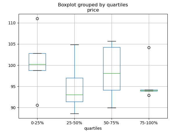
Boxplot for each quartile of a stratifying variable
In [186]: df = pd.DataFrame(
   .....:     {
   .....:         "stratifying_var": np.random.uniform(0, 100, 20),
   .....:         "price": np.random.normal(100, 5, 20),
   .....:     }
   .....: )
   .....:

In [187]: df["quartiles"] = pd.qcut(
   .....:     df["stratifying_var"], 4, labels=["0-25%", "25-50%", "50-75%", "75-100%"]
   .....: )
   .....:

In [188]: df.boxplot(column="price", by="quartiles")
Out[188]: <AxesSubplot:title={'center':'price'}, xlabel='quartiles'>
数据输入/输出#
Performance comparison of SQL vs HDF5
CSV#
这个 CSV 多科
Reading only certain rows of a csv chunk-by-chunk
Reading the first few lines of a frame
读取压缩的文件,但不是 gzip/bz2 (the native compressed formats which read_csv understands). This example shows a WinZipped file, but is a general application of opening the file within a context manager and using that handle to read. See here
处理不良线路 GH2886
Write a multi-row index CSV without writing duplicates
读取多个文件以创建单个DataFrame#
将多个文件合并为单个DataFrame的最佳方法是逐个读取各个帧,将所有单个帧放入一个列表中,然后使用 pd.concat() :
In [189]: for i in range(3):
   .....:     data = pd.DataFrame(np.random.randn(10, 4))
   .....:     data.to_csv("file_{}.csv".format(i))
   .....:

In [190]: files = ["file_0.csv", "file_1.csv", "file_2.csv"]

In [191]: result = pd.concat([pd.read_csv(f) for f in files], ignore_index=True)
您可以使用相同的方法来读取与模式匹配的所有文件。下面是一个使用 glob :
In [192]: import glob

In [193]: import os

In [194]: files = glob.glob("file_*.csv")

In [195]: result = pd.concat([pd.read_csv(f) for f in files], ignore_index=True)
最后,这一策略将与其他策略一起发挥作用 pd.read_*(...) 中所述的功能 io docs 。
解析多列中的日期组件#
使用以下格式可以更快地解析多列中的日期组件
In [196]: i = pd.date_range("20000101", periods=10000)

In [197]: df = pd.DataFrame({"year": i.year, "month": i.month, "day": i.day})

In [198]: df.head()
Out[198]:
   year  month  day
0  2000      1    1
1  2000      1    2
2  2000      1    3
3  2000      1    4
4  2000      1    5

In [199]: %timeit pd.to_datetime(df.year * 10000 + df.month * 100 + df.day, format='%Y%m%d')
   .....: ds = df.apply(lambda x: "%04d%02d%02d" % (x["year"], x["month"], x["day"]), axis=1)
   .....: ds.head()
   .....: %timeit pd.to_datetime(ds)
   .....:
3.4 ms +- 4.03 us per loop (mean +- std. dev. of 7 runs, 100 loops each)
1.19 ms +- 793 ns per loop (mean +- std. dev. of 7 runs, 1,000 loops each)
跳过标题和数据之间的行#
In [200]: data = """;;;;
   .....:  ;;;;
   .....:  ;;;;
   .....:  ;;;;
   .....:  ;;;;
   .....:  ;;;;
   .....: ;;;;
   .....:  ;;;;
   .....:  ;;;;
   .....: ;;;;
   .....: date;Param1;Param2;Param4;Param5
   .....:     ;m²;°C;m²;m
   .....: ;;;;
   .....: 01.01.1990 00:00;1;1;2;3
   .....: 01.01.1990 01:00;5;3;4;5
   .....: 01.01.1990 02:00;9;5;6;7
   .....: 01.01.1990 03:00;13;7;8;9
   .....: 01.01.1990 04:00;17;9;10;11
   .....: 01.01.1990 05:00;21;11;12;13
   .....: """
   .....:
选项1:显式传递行以跳过行#
In [201]: from io import StringIO

In [202]: pd.read_csv(
   .....:     StringIO(data),
   .....:     sep=";",
   .....:     skiprows=[11, 12],
   .....:     index_col=0,
   .....:     parse_dates=True,
   .....:     header=10,
   .....: )
   .....:
Out[202]:
                     Param1  Param2  Param4  Param5
date
1990-01-01 00:00:00       1       1       2       3
1990-01-01 01:00:00       5       3       4       5
1990-01-01 02:00:00       9       5       6       7
1990-01-01 03:00:00      13       7       8       9
1990-01-01 04:00:00      17       9      10      11
1990-01-01 05:00:00      21      11      12      13
选项2:先读取列名,然后读取数据#
In [203]: pd.read_csv(StringIO(data), sep=";", header=10, nrows=10).columns
Out[203]: Index(['date', 'Param1', 'Param2', 'Param4', 'Param5'], dtype='object')

In [204]: columns = pd.read_csv(StringIO(data), sep=";", header=10, nrows=10).columns

In [205]: pd.read_csv(
   .....:     StringIO(data), sep=";", index_col=0, header=12, parse_dates=True, names=columns
   .....: )
   .....:
Out[205]:
                     Param1  Param2  Param4  Param5
date
1990-01-01 00:00:00       1       1       2       3
1990-01-01 01:00:00       5       3       4       5
1990-01-01 02:00:00       9       5       6       7
1990-01-01 03:00:00      13       7       8       9
1990-01-01 04:00:00      17       9      10      11
1990-01-01 05:00:00      21      11      12      13
SQL#
这个 SQL 多科
Excel#
这个 Excel 多科
Reading from a filelike handle
Modifying formatting in XlsxWriter output
仅加载可见的工作表 GH19842#issuecomment-892150745
HTML#
Reading HTML tables from a server that cannot handle the default request header
HDFStore#
这个 HDFStores 多科
Simple queries with a Timestamp Index
使用链接的多表层次结构管理异类数据 GH3032
Merging on-disk tables with millions of rows
Avoiding inconsistencies when writing to a store from multiple processes/threads
按块对大型存储进行重复数据消除,本质上是一种递归缩减操作。显示了一个函数,用于从CSV文件接收数据并按块创建存储,以及日期解析。 See here
Creating a store chunk-by-chunk from a csv file
Appending to a store, while creating a unique index
Reading in a sequence of files, then providing a global unique index to a store while appending
Groupby on a HDFStore with low group density
Groupby on a HDFStore with high group density
Hierarchical queries on a HDFStore
Troubleshoot HDFStore exceptions
Setting min_itemsize with strings
Using ptrepack to create a completely-sorted-index on a store
将属性存储到组节点
In [206]: df = pd.DataFrame(np.random.randn(8, 3))

In [207]: store = pd.HDFStore("test.h5")
---------------------------------------------------------------------------
ModuleNotFoundError                       Traceback (most recent call last)
File /usr/local/lib/python3.10/dist-packages/pandas-1.5.0.dev0+697.gf9762d8f52-py3.10-linux-x86_64.egg/pandas/compat/_optional.py:139, in import_optional_dependency(name, extra, errors, min_version)
    138 try:
--> 139     module = importlib.import_module(name)
    140 except ImportError:

File /usr/lib/python3.10/importlib/__init__.py:126, in import_module(name, package)
    125         level += 1
--> 126 return _bootstrap._gcd_import(name[level:], package, level)

File <frozen importlib._bootstrap>:1050, in _gcd_import(name, package, level)

File <frozen importlib._bootstrap>:1027, in _find_and_load(name, import_)

File <frozen importlib._bootstrap>:1004, in _find_and_load_unlocked(name, import_)

ModuleNotFoundError: No module named 'tables'

During handling of the above exception, another exception occurred:

ImportError                               Traceback (most recent call last)
Input In [207], in <cell line: 1>()
----> 1 store = pd.HDFStore("test.h5")

File /usr/local/lib/python3.10/dist-packages/pandas-1.5.0.dev0+697.gf9762d8f52-py3.10-linux-x86_64.egg/pandas/io/pytables.py:573, in HDFStore.__init__(self, path, mode, complevel, complib, fletcher32, **kwargs)
    570 if "format" in kwargs:
    571     raise ValueError("format is not a defined argument for HDFStore")
--> 573 tables = import_optional_dependency("tables")
    575 if complib is not None and complib not in tables.filters.all_complibs:
    576     raise ValueError(
    577         f"complib only supports {tables.filters.all_complibs} compression."
    578     )

File /usr/local/lib/python3.10/dist-packages/pandas-1.5.0.dev0+697.gf9762d8f52-py3.10-linux-x86_64.egg/pandas/compat/_optional.py:142, in import_optional_dependency(name, extra, errors, min_version)
    140 except ImportError:
    141     if errors == "raise":
--> 142         raise ImportError(msg)
    143     else:
    144         return None

ImportError: Missing optional dependency 'pytables'.  Use pip or conda to install pytables.

In [208]: store.put("df", df)
---------------------------------------------------------------------------
NameError                                 Traceback (most recent call last)
Input In [208], in <cell line: 1>()
----> 1 store.put("df", df)

NameError: name 'store' is not defined

# you can store an arbitrary Python object via pickle
In [209]: store.get_storer("df").attrs.my_attribute = {"A": 10}
---------------------------------------------------------------------------
NameError                                 Traceback (most recent call last)
Input In [209], in <cell line: 1>()
----> 1 store.get_storer("df").attrs.my_attribute = {"A": 10}

NameError: name 'store' is not defined

In [210]: store.get_storer("df").attrs.my_attribute
---------------------------------------------------------------------------
NameError                                 Traceback (most recent call last)
Input In [210], in <cell line: 1>()
----> 1 store.get_storer("df").attrs.my_attribute

NameError: name 'store' is not defined
方法,可以在内存中创建或加载HDFStore driver 参数设置为PyTables。只有在HDFStore关闭时,才会将更改写入磁盘。
In [211]: store = pd.HDFStore("test.h5", "w", driver="H5FD_CORE")
---------------------------------------------------------------------------
ModuleNotFoundError                       Traceback (most recent call last)
File /usr/local/lib/python3.10/dist-packages/pandas-1.5.0.dev0+697.gf9762d8f52-py3.10-linux-x86_64.egg/pandas/compat/_optional.py:139, in import_optional_dependency(name, extra, errors, min_version)
    138 try:
--> 139     module = importlib.import_module(name)
    140 except ImportError:

File /usr/lib/python3.10/importlib/__init__.py:126, in import_module(name, package)
    125         level += 1
--> 126 return _bootstrap._gcd_import(name[level:], package, level)

File <frozen importlib._bootstrap>:1050, in _gcd_import(name, package, level)

File <frozen importlib._bootstrap>:1027, in _find_and_load(name, import_)

File <frozen importlib._bootstrap>:1004, in _find_and_load_unlocked(name, import_)

ModuleNotFoundError: No module named 'tables'

During handling of the above exception, another exception occurred:

ImportError                               Traceback (most recent call last)
Input In [211], in <cell line: 1>()
----> 1 store = pd.HDFStore("test.h5", "w", driver="H5FD_CORE")

File /usr/local/lib/python3.10/dist-packages/pandas-1.5.0.dev0+697.gf9762d8f52-py3.10-linux-x86_64.egg/pandas/io/pytables.py:573, in HDFStore.__init__(self, path, mode, complevel, complib, fletcher32, **kwargs)
    570 if "format" in kwargs:
    571     raise ValueError("format is not a defined argument for HDFStore")
--> 573 tables = import_optional_dependency("tables")
    575 if complib is not None and complib not in tables.filters.all_complibs:
    576     raise ValueError(
    577         f"complib only supports {tables.filters.all_complibs} compression."
    578     )

File /usr/local/lib/python3.10/dist-packages/pandas-1.5.0.dev0+697.gf9762d8f52-py3.10-linux-x86_64.egg/pandas/compat/_optional.py:142, in import_optional_dependency(name, extra, errors, min_version)
    140 except ImportError:
    141     if errors == "raise":
--> 142         raise ImportError(msg)
    143     else:
    144         return None

ImportError: Missing optional dependency 'pytables'.  Use pip or conda to install pytables.

In [212]: df = pd.DataFrame(np.random.randn(8, 3))

In [213]: store["test"] = df
---------------------------------------------------------------------------
NameError                                 Traceback (most recent call last)
Input In [213], in <cell line: 1>()
----> 1 store["test"] = df

NameError: name 'store' is not defined

# only after closing the store, data is written to disk:
In [214]: store.close()
---------------------------------------------------------------------------
NameError                                 Traceback (most recent call last)
Input In [214], in <cell line: 1>()
----> 1 store.close()

NameError: name 'store' is not defined
二进制文件#
如果您需要读入一个由C结构数组组成的二进制文件,Pandas很容易接受NumPy记录数组。例如,假设这个C程序位于一个名为 main.c 编译时使用 gcc main.c -std=gnu99 在64位计算机上,
#include <stdio.h>
#include <stdint.h>

typedef struct _Data
{
    int32_t count;
    double avg;
    float scale;
} Data;

int main(int argc, const char *argv[])
{
    size_t n = 10;
    Data d[n];

    for (int i = 0; i < n; ++i)
    {
        d[i].count = i;
        d[i].avg = i + 1.0;
        d[i].scale = (float) i + 2.0f;
    }

    FILE *file = fopen("binary.dat", "wb");
    fwrite(&d, sizeof(Data), n, file);
    fclose(file);

    return 0;
}
下面的Python代码将读取二进制文件 'binary.dat' 变成了一只Pandas DataFrame ,其中结构的每个元素对应于框架中的一列:
names = "count", "avg", "scale"

# note that the offsets are larger than the size of the type because of
# struct padding
offsets = 0, 8, 16
formats = "i4", "f8", "f4"
dt = np.dtype({"names": names, "offsets": offsets, "formats": formats}, align=True)
df = pd.DataFrame(np.fromfile("binary.dat", dt))
备注
根据在其上创建文件的机器的体系结构,结构元素的偏移量可能不同。不建议将这样的原始二进制文件格式用于常规数据存储,因为它不是跨平台的。我们推荐HDF5或拼花地板,这两种产品都得到了PandasIO设施的支持。
计算#
Numerical integration (sample-based) of a time series
相关性#
通常,获得由以下公式计算的相关矩阵的下(或上)三角形式很有用 DataFrame.corr() 。这可以通过将布尔掩码传递给 where 具体如下:
In [215]: df = pd.DataFrame(np.random.random(size=(100, 5)))

In [216]: corr_mat = df.corr()

In [217]: mask = np.tril(np.ones_like(corr_mat, dtype=np.bool_), k=-1)

In [218]: corr_mat.where(mask)
Out[218]:
          0         1         2        3   4
0       NaN       NaN       NaN      NaN NaN
1 -0.079861       NaN       NaN      NaN NaN
2 -0.236573  0.183801       NaN      NaN NaN
3 -0.013795 -0.051975  0.037235      NaN NaN
4 -0.031974  0.118342 -0.073499 -0.02063 NaN
这个 method argument within DataFrame.corr can accept a callable in addition to the named correlation types. Here we compute the distance correlation 适用于 DataFrame 对象。
In [219]: def distcorr(x, y):
   .....:     n = len(x)
   .....:     a = np.zeros(shape=(n, n))
   .....:     b = np.zeros(shape=(n, n))
   .....:     for i in range(n):
   .....:         for j in range(i + 1, n):
   .....:             a[i, j] = abs(x[i] - x[j])
   .....:             b[i, j] = abs(y[i] - y[j])
   .....:     a += a.T
   .....:     b += b.T
   .....:     a_bar = np.vstack([np.nanmean(a, axis=0)] * n)
   .....:     b_bar = np.vstack([np.nanmean(b, axis=0)] * n)
   .....:     A = a - a_bar - a_bar.T + np.full(shape=(n, n), fill_value=a_bar.mean())
   .....:     B = b - b_bar - b_bar.T + np.full(shape=(n, n), fill_value=b_bar.mean())
   .....:     cov_ab = np.sqrt(np.nansum(A * B)) / n
   .....:     std_a = np.sqrt(np.sqrt(np.nansum(A ** 2)) / n)
   .....:     std_b = np.sqrt(np.sqrt(np.nansum(B ** 2)) / n)
   .....:     return cov_ab / std_a / std_b
   .....:

In [220]: df = pd.DataFrame(np.random.normal(size=(100, 3)))

In [221]: df.corr(method=distcorr)
Out[221]:
          0         1         2
0  1.000000  0.197613  0.216328
1  0.197613  1.000000  0.208749
2  0.216328  0.208749  1.000000
Timedeltas#
这个 Timedeltas 医生。
In [222]: import datetime

In [223]: s = pd.Series(pd.date_range("2012-1-1", periods=3, freq="D"))

In [224]: s - s.max()
Out[224]:
0   -2 days
1   -1 days
2    0 days
dtype: timedelta64[ns]

In [225]: s.max() - s
Out[225]:
0   2 days
1   1 days
2   0 days
dtype: timedelta64[ns]

In [226]: s - datetime.datetime(2011, 1, 1, 3, 5)
Out[226]:
0   364 days 20:55:00
1   365 days 20:55:00
2   366 days 20:55:00
dtype: timedelta64[ns]

In [227]: s + datetime.timedelta(minutes=5)
Out[227]:
0   2012-01-01 00:05:00
1   2012-01-02 00:05:00
2   2012-01-03 00:05:00
dtype: datetime64[ns]

In [228]: datetime.datetime(2011, 1, 1, 3, 5) - s
Out[228]:
0   -365 days +03:05:00
1   -366 days +03:05:00
2   -367 days +03:05:00
dtype: timedelta64[ns]

In [229]: datetime.timedelta(minutes=5) + s
Out[229]:
0   2012-01-01 00:05:00
1   2012-01-02 00:05:00
2   2012-01-03 00:05:00
dtype: datetime64[ns]
Adding and subtracting deltas and dates
In [230]: deltas = pd.Series([datetime.timedelta(days=i) for i in range(3)])

In [231]: df = pd.DataFrame({"A": s, "B": deltas})

In [232]: df
Out[232]:
           A      B
0 2012-01-01 0 days
1 2012-01-02 1 days
2 2012-01-03 2 days

In [233]: df["New Dates"] = df["A"] + df["B"]

In [234]: df["Delta"] = df["A"] - df["New Dates"]

In [235]: df
Out[235]:
           A      B  New Dates   Delta
0 2012-01-01 0 days 2012-01-01  0 days
1 2012-01-02 1 days 2012-01-03 -1 days
2 2012-01-03 2 days 2012-01-05 -2 days

In [236]: df.dtypes
Out[236]:
A             datetime64[ns]
B            timedelta64[ns]
New Dates     datetime64[ns]
Delta        timedelta64[ns]
dtype: object
可以使用np.nan将值设置为NAT,类似于DateTime
In [237]: y = s - s.shift()

In [238]: y
Out[238]:
0      NaT
1   1 days
2   1 days
dtype: timedelta64[ns]

In [239]: y[1] = np.nan

In [240]: y
Out[240]:
0      NaT
1      NaT
2   1 days
dtype: timedelta64[ns]
创建示例数据#
根据某些给定值的任意组合(如R)创建数据帧 expand.grid() 函数,我们可以创建一个DICT,其中键是列名,值是数据值的列表:
In [241]: def expand_grid(data_dict):
   .....:     rows = itertools.product(*data_dict.values())
   .....:     return pd.DataFrame.from_records(rows, columns=data_dict.keys())
   .....:

In [242]: df = expand_grid(
   .....:     {"height": [60, 70], "weight": [100, 140, 180], "sex": ["Male", "Female"]}
   .....: )
   .....:

In [243]: df
Out[243]:
    height  weight     sex
0       60     100    Male
1       60     100  Female
2       60     140    Male
3       60     140  Female
4       60     180    Male
5       60     180  Female
6       70     100    Male
7       70     100  Female
8       70     140    Male
9       70     140  Female
10      70     180    Male
11      70     180  Female