距离Pandas10分钟车程#
这是对Pandas的简短介绍,主要面向新用户。中您可以看到更复杂的食谱 Cookbook 。
通常,我们按如下方式导入:
In [1]: import numpy as np

In [2]: import pandas as pd
对象创建#
请参阅 Intro to data structures section 。
创建一个 Series 通过传递一个值列表,让Pandas创建一个默认的整数索引:
In [3]: s = pd.Series([1, 3, 5, np.nan, 6, 8])

In [4]: s
Out[4]:
0    1.0
1    3.0
2    5.0
3    NaN
4    6.0
5    8.0
dtype: float64
创建一个 DataFrame 通过传递NumPy数组,并使用 date_range() 和带标签的列:
In [5]: dates = pd.date_range("20130101", periods=6)

In [6]: dates
Out[6]:
DatetimeIndex(['2013-01-01', '2013-01-02', '2013-01-03', '2013-01-04',
               '2013-01-05', '2013-01-06'],
              dtype='datetime64[ns]', freq='D')

In [7]: df = pd.DataFrame(np.random.randn(6, 4), index=dates, columns=list("ABCD"))

In [8]: df
Out[8]:
                   A         B         C         D
2013-01-01  0.469112 -0.282863 -1.509059 -1.135632
2013-01-02  1.212112 -0.173215  0.119209 -1.044236
2013-01-03 -0.861849 -2.104569 -0.494929  1.071804
2013-01-04  0.721555 -0.706771 -1.039575  0.271860
2013-01-05 -0.424972  0.567020  0.276232 -1.087401
2013-01-06 -0.673690  0.113648 -1.478427  0.524988
创建一个 DataFrame 通过传递可转换为类似序列的结构的对象的字典:
In [9]: df2 = pd.DataFrame(
   ...:     {
   ...:         "A": 1.0,
   ...:         "B": pd.Timestamp("20130102"),
   ...:         "C": pd.Series(1, index=list(range(4)), dtype="float32"),
   ...:         "D": np.array([3] * 4, dtype="int32"),
   ...:         "E": pd.Categorical(["test", "train", "test", "train"]),
   ...:         "F": "foo",
   ...:     }
   ...: )
   ...:

In [10]: df2
Out[10]:
     A          B    C  D      E    F
0  1.0 2013-01-02  1.0  3   test  foo
1  1.0 2013-01-02  1.0  3  train  foo
2  1.0 2013-01-02  1.0  3   test  foo
3  1.0 2013-01-02  1.0  3  train  foo
In [11]: df2.dtypes
Out[11]:
A           float64
B    datetime64[ns]
C           float32
D             int32
E          category
F            object
dtype: object
如果您使用的是IPython,则会自动启用列名(以及公共属性)的制表符完成功能。以下是将完成的属性的子集:
In [12]: df2.<TAB>  # noqa: E225, E999
df2.A                  df2.bool
df2.abs                df2.boxplot
df2.add                df2.C
df2.add_prefix         df2.clip
df2.add_suffix         df2.columns
df2.align              df2.copy
df2.all                df2.count
df2.any                df2.combine
df2.append             df2.D
df2.apply              df2.describe
df2.applymap           df2.diff
df2.B                  df2.duplicated
如你所见,这些柱子 A , B , C ,以及 D 会自动按Tab键完成。 E 和 F 也存在;为简洁起见,其余属性已被截断。
查看数据#
请参阅 Basics section 。
使用 DataFrame.head() 和 DataFrame.tail() 要分别查看框架的顶行和底行,请执行以下操作:
In [13]: df.head()
Out[13]:
                   A         B         C         D
2013-01-01  0.469112 -0.282863 -1.509059 -1.135632
2013-01-02  1.212112 -0.173215  0.119209 -1.044236
2013-01-03 -0.861849 -2.104569 -0.494929  1.071804
2013-01-04  0.721555 -0.706771 -1.039575  0.271860
2013-01-05 -0.424972  0.567020  0.276232 -1.087401

In [14]: df.tail(3)
Out[14]:
                   A         B         C         D
2013-01-04  0.721555 -0.706771 -1.039575  0.271860
2013-01-05 -0.424972  0.567020  0.276232 -1.087401
2013-01-06 -0.673690  0.113648 -1.478427  0.524988
显示 DataFrame.index 或 DataFrame.columns :
In [15]: df.index
Out[15]:
DatetimeIndex(['2013-01-01', '2013-01-02', '2013-01-03', '2013-01-04',
               '2013-01-05', '2013-01-06'],
              dtype='datetime64[ns]', freq='D')

In [16]: df.columns
Out[16]: Index(['A', 'B', 'C', 'D'], dtype='object')
DataFrame.to_numpy() 给出基础数据的NumPy表示形式。请注意,这可能是一个昂贵的操作,当您 DataFrame 具有不同数据类型的列,这归根结底是Pandas和NumPy之间的根本区别: NumPy数组的整个数组都有一个数据类型,而PandasDataFrame的每列有一个数据类型 。当你打电话的时候 DataFrame.to_numpy() ,Pandas会发现NumPy dtype可以 all DataFrame中的数据类型。这可能最终会是 object ,这需要将每个值强制转换为一个Python对象。
为 df 我们的 DataFrame 在所有浮点值中,以及 DataFrame.to_numpy() 速度快,不需要复制数据:
In [17]: df.to_numpy()
Out[17]:
array([[ 0.4691, -0.2829, -1.5091, -1.1356],
       [ 1.2121, -0.1732,  0.1192, -1.0442],
       [-0.8618, -2.1046, -0.4949,  1.0718],
       [ 0.7216, -0.7068, -1.0396,  0.2719],
       [-0.425 ,  0.567 ,  0.2762, -1.0874],
       [-0.6737,  0.1136, -1.4784,  0.525 ]])
为 df2 ,即 DataFrame 利用多个数据类型, DataFrame.to_numpy() 相对较贵:
In [18]: df2.to_numpy()
Out[18]:
array([[1.0, Timestamp('2013-01-02 00:00:00'), 1.0, 3, 'test', 'foo'],
       [1.0, Timestamp('2013-01-02 00:00:00'), 1.0, 3, 'train', 'foo'],
       [1.0, Timestamp('2013-01-02 00:00:00'), 1.0, 3, 'test', 'foo'],
       [1.0, Timestamp('2013-01-02 00:00:00'), 1.0, 3, 'train', 'foo']],
      dtype=object)
备注
DataFrame.to_numpy() 会吗? not 在输出中包括索引或列标签。
describe() 显示数据的快速统计摘要:
In [19]: df.describe()
Out[19]:
              A         B         C         D
count  6.000000  6.000000  6.000000  6.000000
mean   0.073711 -0.431125 -0.687758 -0.233103
std    0.843157  0.922818  0.779887  0.973118
min   -0.861849 -2.104569 -1.509059 -1.135632
25%   -0.611510 -0.600794 -1.368714 -1.076610
50%    0.022070 -0.228039 -0.767252 -0.386188
75%    0.658444  0.041933 -0.034326  0.461706
max    1.212112  0.567020  0.276232  1.071804
调换您的数据:
In [20]: df.T
Out[20]:
   2013-01-01  2013-01-02  2013-01-03  2013-01-04  2013-01-05  2013-01-06
A    0.469112    1.212112   -0.861849    0.721555   -0.424972   -0.673690
B   -0.282863   -0.173215   -2.104569   -0.706771    0.567020    0.113648
C   -1.509059    0.119209   -0.494929   -1.039575    0.276232   -1.478427
D   -1.135632   -1.044236    1.071804    0.271860   -1.087401    0.524988
DataFrame.sort_index() 按轴排序:
In [21]: df.sort_index(axis=1, ascending=False)
Out[21]:
                   D         C         B         A
2013-01-01 -1.135632 -1.509059 -0.282863  0.469112
2013-01-02 -1.044236  0.119209 -0.173215  1.212112
2013-01-03  1.071804 -0.494929 -2.104569 -0.861849
2013-01-04  0.271860 -1.039575 -0.706771  0.721555
2013-01-05 -1.087401  0.276232  0.567020 -0.424972
2013-01-06  0.524988 -1.478427  0.113648 -0.673690
DataFrame.sort_values() 按值排序:
In [22]: df.sort_values(by="B")
Out[22]:
                   A         B         C         D
2013-01-03 -0.861849 -2.104569 -0.494929  1.071804
2013-01-04  0.721555 -0.706771 -1.039575  0.271860
2013-01-01  0.469112 -0.282863 -1.509059 -1.135632
2013-01-02  1.212112 -0.173215  0.119209 -1.044236
2013-01-06 -0.673690  0.113648 -1.478427  0.524988
2013-01-05 -0.424972  0.567020  0.276232 -1.087401
选择#
备注
虽然用于选择和设置的标准Python/NumPy表达式很直观,并且在交互工作中很方便,但对于生产代码,我们推荐优化的Pandas数据访问方法, DataFrame.at() , DataFrame.iat() , DataFrame.loc() 和 DataFrame.iloc() 。
请参阅索引文档 Indexing and Selecting Data 和 MultiIndex / Advanced Indexing 。
vbl.得到,得到#
选择单个列,这将生成 Series ,相当于 df.A :
In [23]: df["A"]
Out[23]:
2013-01-01    0.469112
2013-01-02    1.212112
2013-01-03   -0.861849
2013-01-04    0.721555
2013-01-05   -0.424972
2013-01-06   -0.673690
Freq: D, Name: A, dtype: float64
Selecting via [] (__getitem__), which slices the rows:
In [24]: df[0:3]
Out[24]:
                   A         B         C         D
2013-01-01  0.469112 -0.282863 -1.509059 -1.135632
2013-01-02  1.212112 -0.173215  0.119209 -1.044236
2013-01-03 -0.861849 -2.104569 -0.494929  1.071804

In [25]: df["20130102":"20130104"]
Out[25]:
                   A         B         C         D
2013-01-02  1.212112 -0.173215  0.119209 -1.044236
2013-01-03 -0.861849 -2.104569 -0.494929  1.071804
2013-01-04  0.721555 -0.706771 -1.039575  0.271860
按标签选择#
有关详细信息,请参阅 Selection by Label 使用 DataFrame.loc() 或 DataFrame.at() 。
要使用标签获取横截面,请执行以下操作:
In [26]: df.loc[dates[0]]
Out[26]:
A    0.469112
B   -0.282863
C   -1.509059
D   -1.135632
Name: 2013-01-01 00:00:00, dtype: float64
按标签在多轴上选择:
In [27]: df.loc[:, ["A", "B"]]
Out[27]:
                   A         B
2013-01-01  0.469112 -0.282863
2013-01-02  1.212112 -0.173215
2013-01-03 -0.861849 -2.104569
2013-01-04  0.721555 -0.706771
2013-01-05 -0.424972  0.567020
2013-01-06 -0.673690  0.113648
显示标签切片,两个端点都是 包括在内 :
In [28]: df.loc["20130102":"20130104", ["A", "B"]]
Out[28]:
                   A         B
2013-01-02  1.212112 -0.173215
2013-01-03 -0.861849 -2.104569
2013-01-04  0.721555 -0.706771
降低返回对象的维度:
In [29]: df.loc["20130102", ["A", "B"]]
Out[29]:
A    1.212112
B   -0.173215
Name: 2013-01-02 00:00:00, dtype: float64
要获取标量值,请执行以下操作:
In [30]: df.loc[dates[0], "A"]
Out[30]: 0.4691122999071863
为了快速访问标量(等同于前面的方法):
In [31]: df.at[dates[0], "A"]
Out[31]: 0.4691122999071863
按位置选择#
有关详细信息,请参阅 Selection by Position 使用 DataFrame.iloc() 或 DataFrame.at() 。
通过传递的整数的位置进行选择:
In [32]: df.iloc[3]
Out[32]:
A    0.721555
B   -0.706771
C   -1.039575
D    0.271860
Name: 2013-01-04 00:00:00, dtype: float64
按整数切片,类似于NumPy/Python:
In [33]: df.iloc[3:5, 0:2]
Out[33]:
                   A         B
2013-01-04  0.721555 -0.706771
2013-01-05 -0.424972  0.567020
按整数位置位置列表,类似于NumPy/Python样式:
In [34]: df.iloc[[1, 2, 4], [0, 2]]
Out[34]:
                   A         C
2013-01-02  1.212112  0.119209
2013-01-03 -0.861849 -0.494929
2013-01-05 -0.424972  0.276232
对于显式切片行:
In [35]: df.iloc[1:3, :]
Out[35]:
                   A         B         C         D
2013-01-02  1.212112 -0.173215  0.119209 -1.044236
2013-01-03 -0.861849 -2.104569 -0.494929  1.071804
对于显式切片列:
In [36]: df.iloc[:, 1:3]
Out[36]:
                   B         C
2013-01-01 -0.282863 -1.509059
2013-01-02 -0.173215  0.119209
2013-01-03 -2.104569 -0.494929
2013-01-04 -0.706771 -1.039575
2013-01-05  0.567020  0.276232
2013-01-06  0.113648 -1.478427
要显式获取值,请执行以下操作:
In [37]: df.iloc[1, 1]
Out[37]: -0.17321464905330858
为了快速访问标量(等同于前面的方法):
In [38]: df.iat[1, 1]
Out[38]: -0.17321464905330858
布尔索引#
使用单个列的值选择数据:
In [39]: df[df["A"] > 0]
Out[39]:
                   A         B         C         D
2013-01-01  0.469112 -0.282863 -1.509059 -1.135632
2013-01-02  1.212112 -0.173215  0.119209 -1.044236
2013-01-04  0.721555 -0.706771 -1.039575  0.271860
从满足布尔条件的DataFrame选择值:
In [40]: df[df > 0]
Out[40]:
                   A         B         C         D
2013-01-01  0.469112       NaN       NaN       NaN
2013-01-02  1.212112       NaN  0.119209       NaN
2013-01-03       NaN       NaN       NaN  1.071804
2013-01-04  0.721555       NaN       NaN  0.271860
2013-01-05       NaN  0.567020  0.276232       NaN
2013-01-06       NaN  0.113648       NaN  0.524988
使用 isin() 过滤方法:
In [41]: df2 = df.copy()

In [42]: df2["E"] = ["one", "one", "two", "three", "four", "three"]

In [43]: df2
Out[43]:
                   A         B         C         D      E
2013-01-01  0.469112 -0.282863 -1.509059 -1.135632    one
2013-01-02  1.212112 -0.173215  0.119209 -1.044236    one
2013-01-03 -0.861849 -2.104569 -0.494929  1.071804    two
2013-01-04  0.721555 -0.706771 -1.039575  0.271860  three
2013-01-05 -0.424972  0.567020  0.276232 -1.087401   four
2013-01-06 -0.673690  0.113648 -1.478427  0.524988  three

In [44]: df2[df2["E"].isin(["two", "four"])]
Out[44]:
                   A         B         C         D     E
2013-01-03 -0.861849 -2.104569 -0.494929  1.071804   two
2013-01-05 -0.424972  0.567020  0.276232 -1.087401  four
设置#
设置新列会自动按索引对齐数据:
In [45]: s1 = pd.Series([1, 2, 3, 4, 5, 6], index=pd.date_range("20130102", periods=6))

In [46]: s1
Out[46]:
2013-01-02    1
2013-01-03    2
2013-01-04    3
2013-01-05    4
2013-01-06    5
2013-01-07    6
Freq: D, dtype: int64

In [47]: df["F"] = s1
按标签设置值:
In [48]: df.at[dates[0], "A"] = 0
按位置设置值:
In [49]: df.iat[0, 1] = 0
通过使用NumPy数组赋值进行设置:
In [50]: df.loc[:, "D"] = np.array([5] * len(df))
先前设置操作的结果:
In [51]: df
Out[51]:
                   A         B         C  D    F
2013-01-01  0.000000  0.000000 -1.509059  5  NaN
2013-01-02  1.212112 -0.173215  0.119209  5  1.0
2013-01-03 -0.861849 -2.104569 -0.494929  5  2.0
2013-01-04  0.721555 -0.706771 -1.039575  5  3.0
2013-01-05 -0.424972  0.567020  0.276232  5  4.0
2013-01-06 -0.673690  0.113648 -1.478427  5  5.0
A where 带设置的操作:
In [52]: df2 = df.copy()

In [53]: df2[df2 > 0] = -df2

In [54]: df2
Out[54]:
                   A         B         C  D    F
2013-01-01  0.000000  0.000000 -1.509059 -5  NaN
2013-01-02 -1.212112 -0.173215 -0.119209 -5 -1.0
2013-01-03 -0.861849 -2.104569 -0.494929 -5 -2.0
2013-01-04 -0.721555 -0.706771 -1.039575 -5 -3.0
2013-01-05 -0.424972 -0.567020 -0.276232 -5 -4.0
2013-01-06 -0.673690 -0.113648 -1.478427 -5 -5.0
缺少数据#
Pandas主要使用的是价值 np.nan 来表示丢失的数据。默认情况下,它不包括在计算中。请参阅 Missing Data section 。
重建索引允许您更改/添加/删除指定轴上的索引。这将返回数据的副本:
In [55]: df1 = df.reindex(index=dates[0:4], columns=list(df.columns) + ["E"])

In [56]: df1.loc[dates[0] : dates[1], "E"] = 1

In [57]: df1
Out[57]:
                   A         B         C  D    F    E
2013-01-01  0.000000  0.000000 -1.509059  5  NaN  1.0
2013-01-02  1.212112 -0.173215  0.119209  5  1.0  1.0
2013-01-03 -0.861849 -2.104569 -0.494929  5  2.0  NaN
2013-01-04  0.721555 -0.706771 -1.039575  5  3.0  NaN
DataFrame.dropna() 删除缺少数据的所有行:
In [58]: df1.dropna(how="any")
Out[58]:
                   A         B         C  D    F    E
2013-01-02  1.212112 -0.173215  0.119209  5  1.0  1.0
DataFrame.fillna() 填充缺失的数据:
In [59]: df1.fillna(value=5)
Out[59]:
                   A         B         C  D    F    E
2013-01-01  0.000000  0.000000 -1.509059  5  5.0  1.0
2013-01-02  1.212112 -0.173215  0.119209  5  1.0  1.0
2013-01-03 -0.861849 -2.104569 -0.494929  5  2.0  5.0
2013-01-04  0.721555 -0.706771 -1.039575  5  3.0  5.0
isna() 获取值所在位置的布尔掩码 nan :
In [60]: pd.isna(df1)
Out[60]:
                A      B      C      D      F      E
2013-01-01  False  False  False  False   True  False
2013-01-02  False  False  False  False  False  False
2013-01-03  False  False  False  False  False   True
2013-01-04  False  False  False  False  False   True
运营#
请参阅 Basic section on Binary Ops 。
统计数据#
总体运营情况 排除 缺少数据。
执行描述性统计:
In [61]: df.mean()
Out[61]:
A   -0.004474
B   -0.383981
C   -0.687758
D    5.000000
F    3.000000
dtype: float64
在另一个轴上执行相同的操作:
In [62]: df.mean(1)
Out[62]:
2013-01-01    0.872735
2013-01-02    1.431621
2013-01-03    0.707731
2013-01-04    1.395042
2013-01-05    1.883656
2013-01-06    1.592306
Freq: D, dtype: float64
操作具有不同维度且需要对齐的对象。此外,Pandas还会自动沿指定维度进行广播:
In [63]: s = pd.Series([1, 3, 5, np.nan, 6, 8], index=dates).shift(2)

In [64]: s
Out[64]:
2013-01-01    NaN
2013-01-02    NaN
2013-01-03    1.0
2013-01-04    3.0
2013-01-05    5.0
2013-01-06    NaN
Freq: D, dtype: float64

In [65]: df.sub(s, axis="index")
Out[65]:
                   A         B         C    D    F
2013-01-01       NaN       NaN       NaN  NaN  NaN
2013-01-02       NaN       NaN       NaN  NaN  NaN
2013-01-03 -1.861849 -3.104569 -1.494929  4.0  1.0
2013-01-04 -2.278445 -3.706771 -4.039575  2.0  0.0
2013-01-05 -5.424972 -4.432980 -4.723768  0.0 -1.0
2013-01-06       NaN       NaN       NaN  NaN  NaN
应用#
DataFrame.apply() 将用户定义的函数应用于数据:
In [66]: df.apply(np.cumsum)
Out[66]:
                   A         B         C   D     F
2013-01-01  0.000000  0.000000 -1.509059   5   NaN
2013-01-02  1.212112 -0.173215 -1.389850  10   1.0
2013-01-03  0.350263 -2.277784 -1.884779  15   3.0
2013-01-04  1.071818 -2.984555 -2.924354  20   6.0
2013-01-05  0.646846 -2.417535 -2.648122  25  10.0
2013-01-06 -0.026844 -2.303886 -4.126549  30  15.0

In [67]: df.apply(lambda x: x.max() - x.min())
Out[67]:
A    2.073961
B    2.671590
C    1.785291
D    0.000000
F    4.000000
dtype: float64
组织构图#
见更多 Histogramming and Discretization 。
In [68]: s = pd.Series(np.random.randint(0, 7, size=10))

In [69]: s
Out[69]:
0    4
1    2
2    1
3    2
4    6
5    4
6    4
7    6
8    4
9    4
dtype: int64

In [70]: s.value_counts()
Out[70]:
4    5
2    2
6    2
1    1
dtype: int64
字符串方法#
系列中配备了一组字符串处理方法。 str attribute that make it easy to operate on each element of the array, as in the code snippet below. Note that pattern-matching in str generally uses regular expressions 默认情况下(在某些情况下总是使用它们)。见更多 Vectorized String Methods 。
In [71]: s = pd.Series(["A", "B", "C", "Aaba", "Baca", np.nan, "CABA", "dog", "cat"])

In [72]: s.str.lower()
Out[72]:
0       a
1       b
2       c
3    aaba
4    baca
5     NaN
6    caba
7     dog
8     cat
dtype: object
合并#
合并#
Pandas提供了各种工具,可以轻松地将Series和DataFrame对象与索引的各种集合逻辑组合在一起,并在连接/合并类型的操作中使用关系代数功能。
请参阅 Merging section 。
将Pandas物体沿着一条轴连接在一起 concat() :
In [73]: df = pd.DataFrame(np.random.randn(10, 4))

In [74]: df
Out[74]:
          0         1         2         3
0 -0.548702  1.467327 -1.015962 -0.483075
1  1.637550 -1.217659 -0.291519 -1.745505
2 -0.263952  0.991460 -0.919069  0.266046
3 -0.709661  1.669052  1.037882 -1.705775
4 -0.919854 -0.042379  1.247642 -0.009920
5  0.290213  0.495767  0.362949  1.548106
6 -1.131345 -0.089329  0.337863 -0.945867
7 -0.932132  1.956030  0.017587 -0.016692
8 -0.575247  0.254161 -1.143704  0.215897
9  1.193555 -0.077118 -0.408530 -0.862495

# break it into pieces
In [75]: pieces = [df[:3], df[3:7], df[7:]]

In [76]: pd.concat(pieces)
Out[76]:
          0         1         2         3
0 -0.548702  1.467327 -1.015962 -0.483075
1  1.637550 -1.217659 -0.291519 -1.745505
2 -0.263952  0.991460 -0.919069  0.266046
3 -0.709661  1.669052  1.037882 -1.705775
4 -0.919854 -0.042379  1.247642 -0.009920
5  0.290213  0.495767  0.362949  1.548106
6 -1.131345 -0.089329  0.337863 -0.945867
7 -0.932132  1.956030  0.017587 -0.016692
8 -0.575247  0.254161 -1.143704  0.215897
9  1.193555 -0.077118 -0.408530 -0.862495
会合#
merge() 启用沿特定列的SQL样式联接类型。请参阅 Database style joining 部分。
In [77]: left = pd.DataFrame({"key": ["foo", "foo"], "lval": [1, 2]})

In [78]: right = pd.DataFrame({"key": ["foo", "foo"], "rval": [4, 5]})

In [79]: left
Out[79]:
   key  lval
0  foo     1
1  foo     2

In [80]: right
Out[80]:
   key  rval
0  foo     4
1  foo     5

In [81]: pd.merge(left, right, on="key")
Out[81]:
   key  lval  rval
0  foo     1     4
1  foo     1     5
2  foo     2     4
3  foo     2     5
另一个可以举的例子是:
In [82]: left = pd.DataFrame({"key": ["foo", "bar"], "lval": [1, 2]})

In [83]: right = pd.DataFrame({"key": ["foo", "bar"], "rval": [4, 5]})

In [84]: left
Out[84]:
   key  lval
0  foo     1
1  bar     2

In [85]: right
Out[85]:
   key  rval
0  foo     4
1  bar     5

In [86]: pd.merge(left, right, on="key")
Out[86]:
   key  lval  rval
0  foo     1     4
1  bar     2     5
分组#
我们所说的“分组依据”是指涉及以下一个或多个步骤的过程:
拆分 根据某些标准将数据分组
施药 独立于每一组的函数
组合 将结果转换为数据结构
请参阅 Grouping section 。
In [87]: df = pd.DataFrame(
   ....:     {
   ....:         "A": ["foo", "bar", "foo", "bar", "foo", "bar", "foo", "foo"],
   ....:         "B": ["one", "one", "two", "three", "two", "two", "one", "three"],
   ....:         "C": np.random.randn(8),
   ....:         "D": np.random.randn(8),
   ....:     }
   ....: )
   ....:

In [88]: df
Out[88]:
     A      B         C         D
0  foo    one  1.346061 -1.577585
1  bar    one  1.511763  0.396823
2  foo    two  1.627081 -0.105381
3  bar  three -0.990582 -0.532532
4  foo    two -0.441652  1.453749
5  bar    two  1.211526  1.208843
6  foo    one  0.268520 -0.080952
7  foo  three  0.024580 -0.264610
分组,然后应用 sum() 函数应用于所产生的组:
In [89]: df.groupby("A").sum()
Out[89]:
            C         D
A
bar  1.732707  1.073134
foo  2.824590 -0.574779
按多列分组形成了分层索引,我们可以再次应用 sum() 功能:
In [90]: df.groupby(["A", "B"]).sum()
Out[90]:
                  C         D
A   B
bar one    1.511763  0.396823
    three -0.990582 -0.532532
    two    1.211526  1.208843
foo one    1.614581 -1.658537
    three  0.024580 -0.264610
    two    1.185429  1.348368
重塑#
请参阅上的部分 Hierarchical Indexing 和 Reshaping 。
栈#
In [91]: tuples = list(
   ....:     zip(
   ....:         ["bar", "bar", "baz", "baz", "foo", "foo", "qux", "qux"],
   ....:         ["one", "two", "one", "two", "one", "two", "one", "two"],
   ....:     )
   ....: )
   ....:

In [92]: index = pd.MultiIndex.from_tuples(tuples, names=["first", "second"])

In [93]: df = pd.DataFrame(np.random.randn(8, 2), index=index, columns=["A", "B"])

In [94]: df2 = df[:4]

In [95]: df2
Out[95]:
                     A         B
first second
bar   one    -0.727965 -0.589346
      two     0.339969 -0.693205
baz   one    -0.339355  0.593616
      two     0.884345  1.591431
这个 stack() 方法“压缩”DataFrame列中的一个级别:
In [96]: stacked = df2.stack()

In [97]: stacked
Out[97]:
first  second
bar    one     A   -0.727965
               B   -0.589346
       two     A    0.339969
               B   -0.693205
baz    one     A   -0.339355
               B    0.593616
       two     A    0.884345
               B    1.591431
dtype: float64
具有“堆叠”的DataFrame或Series(具有 MultiIndex 作为 index )的逆运算。 stack() 是 unstack() ,这在默认情况下会将 最后一关 :
In [98]: stacked.unstack()
Out[98]:
                     A         B
first second
bar   one    -0.727965 -0.589346
      two     0.339969 -0.693205
baz   one    -0.339355  0.593616
      two     0.884345  1.591431

In [99]: stacked.unstack(1)
Out[99]:
second        one       two
first
bar   A -0.727965  0.339969
      B -0.589346 -0.693205
baz   A -0.339355  0.884345
      B  0.593616  1.591431

In [100]: stacked.unstack(0)
Out[100]:
first          bar       baz
second
one    A -0.727965 -0.339355
       B -0.589346  0.593616
two    A  0.339969  0.884345
       B -0.693205  1.591431
数据透视表#
请参阅 Pivot Tables 。
In [101]: df = pd.DataFrame(
   .....:     {
   .....:         "A": ["one", "one", "two", "three"] * 3,
   .....:         "B": ["A", "B", "C"] * 4,
   .....:         "C": ["foo", "foo", "foo", "bar", "bar", "bar"] * 2,
   .....:         "D": np.random.randn(12),
   .....:         "E": np.random.randn(12),
   .....:     }
   .....: )
   .....:

In [102]: df
Out[102]:
        A  B    C         D         E
0     one  A  foo -1.202872  0.047609
1     one  B  foo -1.814470 -0.136473
2     two  C  foo  1.018601 -0.561757
3   three  A  bar -0.595447 -1.623033
4     one  B  bar  1.395433  0.029399
5     one  C  bar -0.392670 -0.542108
6     two  A  foo  0.007207  0.282696
7   three  B  foo  1.928123 -0.087302
8     one  C  foo -0.055224 -1.575170
9     one  A  bar  2.395985  1.771208
10    two  B  bar  1.552825  0.816482
11  three  C  bar  0.166599  1.100230
pivot_table() pivots a DataFrame specifying the values, index and columns
In [103]: pd.pivot_table(df, values="D", index=["A", "B"], columns=["C"])
Out[103]:
C             bar       foo
A     B
one   A  2.395985 -1.202872
      B  1.395433 -1.814470
      C -0.392670 -0.055224
three A -0.595447       NaN
      B       NaN  1.928123
      C  0.166599       NaN
two   A       NaN  0.007207
      B  1.552825       NaN
      C       NaN  1.018601
时间序列#
Pandas具有简单、强大和高效的功能,可以在频率转换期间执行重采样操作(例如,将第二个数据转换为5分钟的数据)。这在金融应用程序中非常常见,但不限于此。请参阅 Time Series section 。
In [104]: rng = pd.date_range("1/1/2012", periods=100, freq="S")

In [105]: ts = pd.Series(np.random.randint(0, 500, len(rng)), index=rng)

In [106]: ts.resample("5Min").sum()
Out[106]:
2012-01-01    24182
Freq: 5T, dtype: int64
Series.tz_localize() 将时间序列本地化到时区:
In [107]: rng = pd.date_range("3/6/2012 00:00", periods=5, freq="D")

In [108]: ts = pd.Series(np.random.randn(len(rng)), rng)

In [109]: ts
Out[109]:
2012-03-06    1.857704
2012-03-07   -1.193545
2012-03-08    0.677510
2012-03-09   -0.153931
2012-03-10    0.520091
Freq: D, dtype: float64

In [110]: ts_utc = ts.tz_localize("UTC")

In [111]: ts_utc
Out[111]:
2012-03-06 00:00:00+00:00    1.857704
2012-03-07 00:00:00+00:00   -1.193545
2012-03-08 00:00:00+00:00    0.677510
2012-03-09 00:00:00+00:00   -0.153931
2012-03-10 00:00:00+00:00    0.520091
Freq: D, dtype: float64
Series.tz_convert() 将时区感知的时间序列转换为另一个时区:
In [112]: ts_utc.tz_convert("US/Eastern")
Out[112]:
2012-03-05 19:00:00-05:00    1.857704
2012-03-06 19:00:00-05:00   -1.193545
2012-03-07 19:00:00-05:00    0.677510
2012-03-08 19:00:00-05:00   -0.153931
2012-03-09 19:00:00-05:00    0.520091
Freq: D, dtype: float64
在时间跨度表示法之间转换:
In [113]: rng = pd.date_range("1/1/2012", periods=5, freq="M")

In [114]: ts = pd.Series(np.random.randn(len(rng)), index=rng)

In [115]: ts
Out[115]:
2012-01-31   -1.475051
2012-02-29    0.722570
2012-03-31   -0.322646
2012-04-30   -1.601631
2012-05-31    0.778033
Freq: M, dtype: float64

In [116]: ps = ts.to_period()

In [117]: ps
Out[117]:
2012-01   -1.475051
2012-02    0.722570
2012-03   -0.322646
2012-04   -1.601631
2012-05    0.778033
Freq: M, dtype: float64

In [118]: ps.to_timestamp()
Out[118]:
2012-01-01   -1.475051
2012-02-01    0.722570
2012-03-01   -0.322646
2012-04-01   -1.601631
2012-05-01    0.778033
Freq: MS, dtype: float64
在PERIOD和TIMESTAMP之间进行转换可以使用一些方便的算术函数。在下面的示例中,我们将年度结束时间为11月的季度频率转换为季度结束后的下一个月的上午9点:
In [119]: prng = pd.period_range("1990Q1", "2000Q4", freq="Q-NOV")

In [120]: ts = pd.Series(np.random.randn(len(prng)), prng)

In [121]: ts.index = (prng.asfreq("M", "e") + 1).asfreq("H", "s") + 9

In [122]: ts.head()
Out[122]:
1990-03-01 09:00   -0.289342
1990-06-01 09:00    0.233141
1990-09-01 09:00   -0.223540
1990-12-01 09:00    0.542054
1991-03-01 09:00   -0.688585
Freq: H, dtype: float64
类别词#
Pandas可以将分类数据包含在 DataFrame 。有关完整的文档,请参阅 categorical introduction 以及 API documentation 。
In [123]: df = pd.DataFrame(
   .....:     {"id": [1, 2, 3, 4, 5, 6], "raw_grade": ["a", "b", "b", "a", "a", "e"]}
   .....: )
   .....:
将原始分数转换为分类数据类型:
In [124]: df["grade"] = df["raw_grade"].astype("category")

In [125]: df["grade"]
Out[125]:
0    a
1    b
2    b
3    a
4    a
5    e
Name: grade, dtype: category
Categories (3, object): ['a', 'b', 'e']
将类别重命名为更有意义的名称(分配给 Series.cat.categories() 已就位!):
In [126]: df["grade"].cat.categories = ["very good", "good", "very bad"]
重新排序类别并同时添加缺少的类别(方法位于 Series.cat() 返回一个新的 Series 默认情况下):
In [127]: df["grade"] = df["grade"].cat.set_categories(
   .....:     ["very bad", "bad", "medium", "good", "very good"]
   .....: )
   .....:

In [128]: df["grade"]
Out[128]:
0    very good
1         good
2         good
3    very good
4    very good
5     very bad
Name: grade, dtype: category
Categories (5, object): ['very bad', 'bad', 'medium', 'good', 'very good']
排序是按类别的顺序进行的,而不是按词汇顺序:
In [129]: df.sort_values(by="grade")
Out[129]:
   id raw_grade      grade
5   6         e   very bad
1   2         b       good
2   3         b       good
0   1         a  very good
3   4         a  very good
4   5         a  very good
按分类列分组还会显示空类别:
In [130]: df.groupby("grade").size()
Out[130]:
grade
very bad     1
bad          0
medium       0
good         2
very good    3
dtype: int64
标绘#
请参阅 Plotting 医生。
我们使用标准约定来引用matplotlib API:
In [131]: import matplotlib.pyplot as plt

In [132]: plt.close("all")
这个 plt.close method is used to close 图形窗口:
In [133]: ts = pd.Series(np.random.randn(1000), index=pd.date_range("1/1/2000", periods=1000))

In [134]: ts = ts.cumsum()

In [135]: ts.plot();
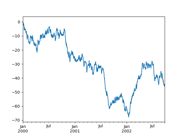
如果在Jupyter Notebook下运行,曲线图将显示在 plot() 。否则请使用 matplotlib.pyplot.show 展示它,或者 matplotlib.pyplot.savefig 将其写入文件。
In [136]: plt.show();
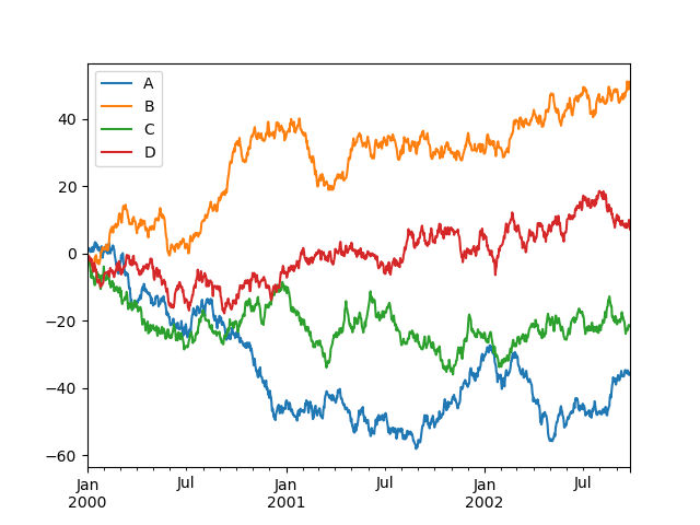
在DataFrame上, plot() 方法可以方便地绘制带有标签的所有列:
In [137]: df = pd.DataFrame(
   .....:     np.random.randn(1000, 4), index=ts.index, columns=["A", "B", "C", "D"]
   .....: )
   .....:

In [138]: df = df.cumsum()

In [139]: plt.figure();

In [140]: df.plot();

In [141]: plt.legend(loc='best');
导入和导出数据#
CSV#
Writing to a csv file: using DataFrame.to_csv()
In [142]: df.to_csv("foo.csv")
Reading from a csv file: using read_csv()
In [143]: pd.read_csv("foo.csv")
Out[143]:
     Unnamed: 0          A          B          C          D
0    2000-01-01   0.350262   0.843315   1.798556   0.782234
1    2000-01-02  -0.586873   0.034907   1.923792  -0.562651
2    2000-01-03  -1.245477  -0.963406   2.269575  -1.612566
3    2000-01-04  -0.252830  -0.498066   3.176886  -1.275581
4    2000-01-05  -1.044057   0.118042   2.768571   0.386039
..          ...        ...        ...        ...        ...
995  2002-09-22 -48.017654  31.474551  69.146374 -47.541670
996  2002-09-23 -47.207912  32.627390  68.505254 -48.828331
997  2002-09-24 -48.907133  31.990402  67.310924 -49.391051
998  2002-09-25 -50.146062  33.716770  67.717434 -49.037577
999  2002-09-26 -49.724318  33.479952  68.108014 -48.822030

[1000 rows x 5 columns]
HDF5#
读取和写入到 HDFStores 。
使用以下命令写入HDF5存储 DataFrame.to_hdf() :
In [144]: df.to_hdf("foo.h5", "df")
---------------------------------------------------------------------------
ModuleNotFoundError                       Traceback (most recent call last)
File /usr/local/lib/python3.10/dist-packages/pandas-1.5.0.dev0+697.gf9762d8f52-py3.10-linux-x86_64.egg/pandas/compat/_optional.py:139, in import_optional_dependency(name, extra, errors, min_version)
    138 try:
--> 139     module = importlib.import_module(name)
    140 except ImportError:

File /usr/lib/python3.10/importlib/__init__.py:126, in import_module(name, package)
    125         level += 1
--> 126 return _bootstrap._gcd_import(name[level:], package, level)

File <frozen importlib._bootstrap>:1050, in _gcd_import(name, package, level)

File <frozen importlib._bootstrap>:1027, in _find_and_load(name, import_)

File <frozen importlib._bootstrap>:1004, in _find_and_load_unlocked(name, import_)

ModuleNotFoundError: No module named 'tables'

During handling of the above exception, another exception occurred:

ImportError                               Traceback (most recent call last)
Input In [144], in <cell line: 1>()
----> 1 df.to_hdf("foo.h5", "df")

File /usr/local/lib/python3.10/dist-packages/pandas-1.5.0.dev0+697.gf9762d8f52-py3.10-linux-x86_64.egg/pandas/core/generic.py:2655, in NDFrame.to_hdf(self, path_or_buf, key, mode, complevel, complib, append, format, index, min_itemsize, nan_rep, dropna, data_columns, errors, encoding)
   2651 from pandas.io import pytables
   2653 # Argument 3 to "to_hdf" has incompatible type "NDFrame"; expected
   2654 # "Union[DataFrame, Series]" [arg-type]
-> 2655 pytables.to_hdf(
   2656     path_or_buf,
   2657     key,
   2658     self,  # type: ignore[arg-type]
   2659     mode=mode,
   2660     complevel=complevel,
   2661     complib=complib,
   2662     append=append,
   2663     format=format,
   2664     index=index,
   2665     min_itemsize=min_itemsize,
   2666     nan_rep=nan_rep,
   2667     dropna=dropna,
   2668     data_columns=data_columns,
   2669     errors=errors,
   2670     encoding=encoding,
   2671 )

File /usr/local/lib/python3.10/dist-packages/pandas-1.5.0.dev0+697.gf9762d8f52-py3.10-linux-x86_64.egg/pandas/io/pytables.py:312, in to_hdf(path_or_buf, key, value, mode, complevel, complib, append, format, index, min_itemsize, nan_rep, dropna, data_columns, errors, encoding)
    310 path_or_buf = stringify_path(path_or_buf)
    311 if isinstance(path_or_buf, str):
--> 312     with HDFStore(
    313         path_or_buf, mode=mode, complevel=complevel, complib=complib
    314     ) as store:
    315         f(store)
    316 else:

File /usr/local/lib/python3.10/dist-packages/pandas-1.5.0.dev0+697.gf9762d8f52-py3.10-linux-x86_64.egg/pandas/io/pytables.py:573, in HDFStore.__init__(self, path, mode, complevel, complib, fletcher32, **kwargs)
    570 if "format" in kwargs:
    571     raise ValueError("format is not a defined argument for HDFStore")
--> 573 tables = import_optional_dependency("tables")
    575 if complib is not None and complib not in tables.filters.all_complibs:
    576     raise ValueError(
    577         f"complib only supports {tables.filters.all_complibs} compression."
    578     )

File /usr/local/lib/python3.10/dist-packages/pandas-1.5.0.dev0+697.gf9762d8f52-py3.10-linux-x86_64.egg/pandas/compat/_optional.py:142, in import_optional_dependency(name, extra, errors, min_version)
    140 except ImportError:
    141     if errors == "raise":
--> 142         raise ImportError(msg)
    143     else:
    144         return None

ImportError: Missing optional dependency 'pytables'.  Use pip or conda to install pytables.
使用以下命令从HDF5商店读取 read_hdf() :
In [145]: pd.read_hdf("foo.h5", "df")
---------------------------------------------------------------------------
FileNotFoundError                         Traceback (most recent call last)
Input In [145], in <cell line: 1>()
----> 1 pd.read_hdf("foo.h5", "df")

File /usr/local/lib/python3.10/dist-packages/pandas-1.5.0.dev0+697.gf9762d8f52-py3.10-linux-x86_64.egg/pandas/io/pytables.py:428, in read_hdf(path_or_buf, key, mode, errors, where, start, stop, columns, iterator, chunksize, **kwargs)
    425     exists = False
    427 if not exists:
--> 428     raise FileNotFoundError(f"File {path_or_buf} does not exist")
    430 store = HDFStore(path_or_buf, mode=mode, errors=errors, **kwargs)
    431 # can't auto open/close if we are using an iterator
    432 # so delegate to the iterator

FileNotFoundError: File foo.h5 does not exist
Excel#
读取和写入到 Excel 。
使用写入到Excel文件 DataFrame.to_excel() :
In [146]: df.to_excel("foo.xlsx", sheet_name="Sheet1")
---------------------------------------------------------------------------
ModuleNotFoundError                       Traceback (most recent call last)
Input In [146], in <cell line: 1>()
----> 1 df.to_excel("foo.xlsx", sheet_name="Sheet1")

File /usr/local/lib/python3.10/dist-packages/pandas-1.5.0.dev0+697.gf9762d8f52-py3.10-linux-x86_64.egg/pandas/core/generic.py:2237, in NDFrame.to_excel(self, excel_writer, sheet_name, na_rep, float_format, columns, header, index, index_label, startrow, startcol, engine, merge_cells, encoding, inf_rep, verbose, freeze_panes, storage_options)
   2224 from pandas.io.formats.excel import ExcelFormatter
   2226 formatter = ExcelFormatter(
   2227     df,
   2228     na_rep=na_rep,
   (...)
   2235     inf_rep=inf_rep,
   2236 )
-> 2237 formatter.write(
   2238     excel_writer,
   2239     sheet_name=sheet_name,
   2240     startrow=startrow,
   2241     startcol=startcol,
   2242     freeze_panes=freeze_panes,
   2243     engine=engine,
   2244     storage_options=storage_options,
   2245 )

File /usr/local/lib/python3.10/dist-packages/pandas-1.5.0.dev0+697.gf9762d8f52-py3.10-linux-x86_64.egg/pandas/io/formats/excel.py:896, in ExcelFormatter.write(self, writer, sheet_name, startrow, startcol, freeze_panes, engine, storage_options)
    892     need_save = False
    893 else:
    894     # error: Cannot instantiate abstract class 'ExcelWriter' with abstract
    895     # attributes 'engine', 'save', 'supported_extensions' and 'write_cells'
--> 896     writer = ExcelWriter(  # type: ignore[abstract]
    897         writer, engine=engine, storage_options=storage_options
    898     )
    899     need_save = True
    901 try:

File /usr/local/lib/python3.10/dist-packages/pandas-1.5.0.dev0+697.gf9762d8f52-py3.10-linux-x86_64.egg/pandas/io/excel/_openpyxl.py:55, in OpenpyxlWriter.__init__(self, path, engine, date_format, datetime_format, mode, storage_options, if_sheet_exists, engine_kwargs, **kwargs)
     42 def __init__(
     43     self,
     44     path: FilePath | WriteExcelBuffer | ExcelWriter,
   (...)
     53 ) -> None:
     54     # Use the openpyxl module as the Excel writer.
---> 55     from openpyxl.workbook import Workbook
     57     engine_kwargs = combine_kwargs(engine_kwargs, kwargs)
     59     super().__init__(
     60         path,
     61         mode=mode,
   (...)
     64         engine_kwargs=engine_kwargs,
     65     )

ModuleNotFoundError: No module named 'openpyxl'
使用从Excel文件中读取 read_excel() :
In [147]: pd.read_excel("foo.xlsx", "Sheet1", index_col=None, na_values=["NA"])
---------------------------------------------------------------------------
FileNotFoundError                         Traceback (most recent call last)
Input In [147], in <cell line: 1>()
----> 1 pd.read_excel("foo.xlsx", "Sheet1", index_col=None, na_values=["NA"])

File /usr/local/lib/python3.10/dist-packages/pandas-1.5.0.dev0+697.gf9762d8f52-py3.10-linux-x86_64.egg/pandas/util/_decorators.py:317, in deprecate_nonkeyword_arguments.<locals>.decorate.<locals>.wrapper(*args, **kwargs)
    311 if len(args) > num_allow_args:
    312     warnings.warn(
    313         msg.format(arguments=arguments),
    314         FutureWarning,
    315         stacklevel=stacklevel,
    316     )
--> 317 return func(*args, **kwargs)

File /usr/local/lib/python3.10/dist-packages/pandas-1.5.0.dev0+697.gf9762d8f52-py3.10-linux-x86_64.egg/pandas/io/excel/_base.py:458, in read_excel(io, sheet_name, header, names, index_col, usecols, squeeze, dtype, engine, converters, true_values, false_values, skiprows, nrows, na_values, keep_default_na, na_filter, verbose, parse_dates, date_parser, thousands, decimal, comment, skipfooter, convert_float, mangle_dupe_cols, storage_options)
    456 if not isinstance(io, ExcelFile):
    457     should_close = True
--> 458     io = ExcelFile(io, storage_options=storage_options, engine=engine)
    459 elif engine and engine != io.engine:
    460     raise ValueError(
    461         "Engine should not be specified when passing "
    462         "an ExcelFile - ExcelFile already has the engine set"
    463     )

File /usr/local/lib/python3.10/dist-packages/pandas-1.5.0.dev0+697.gf9762d8f52-py3.10-linux-x86_64.egg/pandas/io/excel/_base.py:1482, in ExcelFile.__init__(self, path_or_buffer, engine, storage_options)
   1480     ext = "xls"
   1481 else:
-> 1482     ext = inspect_excel_format(
   1483         content_or_path=path_or_buffer, storage_options=storage_options
   1484     )
   1485     if ext is None:
   1486         raise ValueError(
   1487             "Excel file format cannot be determined, you must specify "
   1488             "an engine manually."
   1489         )

File /usr/local/lib/python3.10/dist-packages/pandas-1.5.0.dev0+697.gf9762d8f52-py3.10-linux-x86_64.egg/pandas/io/excel/_base.py:1355, in inspect_excel_format(content_or_path, storage_options)
   1352 if isinstance(content_or_path, bytes):
   1353     content_or_path = BytesIO(content_or_path)
-> 1355 with get_handle(
   1356     content_or_path, "rb", storage_options=storage_options, is_text=False
   1357 ) as handle:
   1358     stream = handle.handle
   1359     stream.seek(0)

File /usr/local/lib/python3.10/dist-packages/pandas-1.5.0.dev0+697.gf9762d8f52-py3.10-linux-x86_64.egg/pandas/io/common.py:795, in get_handle(path_or_buf, mode, encoding, compression, memory_map, is_text, errors, storage_options)
    786         handle = open(
    787             handle,
    788             ioargs.mode,
   (...)
    791             newline="",
    792         )
    793     else:
    794         # Binary mode
--> 795         handle = open(handle, ioargs.mode)
    796     handles.append(handle)
    798 # Convert BytesIO or file objects passed with an encoding

FileNotFoundError: [Errno 2] No such file or directory: 'foo.xlsx'
我明白了#
如果您正尝试对 Series 或 DataFrame 您可能会看到一个例外,如:
In [148]: if pd.Series([False, True, False]):
   .....:      print("I was true")
   .....:
---------------------------------------------------------------------------
ValueError                                Traceback (most recent call last)
Input In [148], in <cell line: 1>()
----> 1 if pd.Series([False, True, False]):
      2      print("I was true")

File /usr/local/lib/python3.10/dist-packages/pandas-1.5.0.dev0+697.gf9762d8f52-py3.10-linux-x86_64.egg/pandas/core/generic.py:1417, in NDFrame.__nonzero__(self)
   1415 @final
   1416 def __nonzero__(self):
-> 1417     raise ValueError(
   1418         f"The truth value of a {type(self).__name__} is ambiguous. "
   1419         "Use a.empty, a.bool(), a.item(), a.any() or a.all()."
   1420     )

ValueError: The truth value of a Series is ambiguous. Use a.empty, a.bool(), a.item(), a.any() or a.all().
看见 Comparisons 和 Gotchas 想要一个解释和该怎么做。