备注
GeoPandas简介#
本快速教程介绍了GeoPandas的主要概念和基本功能,以帮助您开始您的项目。
概念#
GeoPandas,顾名思义,扩展了科普数据科学库 pandas 通过添加对地理空间数据的支持。如果您不熟悉 pandas, we recommend taking a quick look at its Getting started documentation 在继续之前。
GeoPandas中的核心数据结构是 geopandas.GeoDataFrame ,是的子类 pandas.DataFrame ,它可以存储几何图形列并执行空间操作。这个 geopandas.GeoSeries ,是的子类 pandas.Series 处理几何图形。因此,您的 GeoDataFrame 是一种组合 pandas.Series ,以及传统数据(数字、布尔、文本等),以及 geopandas.GeoSeries ,使用几何图形(点、多边形等)。您可以拥有任意数量的带有几何图形的列;桌面GIS软件没有典型的限制。

每个人 GeoSeries 可以包含任何几何类型(甚至可以在单个数组中混合它们),并且具有 GeoSeries.crs 属性,该属性存储有关投影的信息(CRS代表坐标参考系)。因此,每个 GeoSeries 在一个 GeoDataFrame 可以在不同的投影中,例如,允许您拥有同一几何体的多个版本(不同的投影)。
只有一个 GeoSeries 在一个 GeoDataFrame 被认为是 活动的 几何图形,这意味着所有几何运算都应用于 GeoDataFrame 对此进行操作 活动的 列。
用户指南
请参阅更多信息 data structures in the User Guide 。
让我们看看其中一些概念是如何在实践中发挥作用的。
读取和写入文件#
首先,我们需要读取一些数据。
正在读取文件#
假设您有一个同时包含数据和几何的文件(例如,GeoPackage、GeoJSON、shapefile),则可以使用 geopandas.read_file() ,它会自动检测文件类型并创建 GeoDataFrame 。本教程使用 "nybb" 数据集,纽约区地图,是GeoPandas安装的一部分。因此,我们使用 geopandas.datasets.get_path() 以检索数据集的路径。
[1]:
import geopandas

path_to_data = geopandas.datasets.get_path("nybb")
gdf = geopandas.read_file(path_to_data)

gdf
[1]:
| BoroCode | BoroName | Shape_Leng | Shape_Area | geometry | |
|---|---|---|---|---|---|
| 0 | 5 | Staten Island | 330470.010332 | 1.623820e+09 | MULTIPOLYGON (((970217.022 145643.332, 970227.... |
| 1 | 4 | Queens | 896344.047763 | 3.045213e+09 | MULTIPOLYGON (((1029606.077 156073.814, 102957... |
| 2 | 3 | Brooklyn | 741080.523166 | 1.937479e+09 | MULTIPOLYGON (((1021176.479 151374.797, 102100... |
| 3 | 1 | Manhattan | 359299.096471 | 6.364715e+08 | MULTIPOLYGON (((981219.056 188655.316, 980940.... |
| 4 | 2 | Bronx | 464392.991824 | 1.186925e+09 | MULTIPOLYGON (((1012821.806 229228.265, 101278... |
正在写入文件#
要编写一个 GeoDataFrame 返回文件使用 GeoDataFrame.to_file() 。默认文件格式为shapefile,但您可以使用 driver 关键字。
[2]:
gdf.to_file("my_file.geojson", driver="GeoJSON")
用户指南
简单的访问器和方法#
现在我们有了我们的 GeoDataFrame 并且可以开始使用它的几何体。
由于纽约区数据集中只有一个几何列,因此该列自动成为 活动的 使用的几何和空间方法 GeoDataFrame 将应用于 "geometry" 列。
测量面积#
要测量每个多边形(或在此特定情况下为多个多边形)的面积,请访问 GeoDataFrame.area 属性,该属性返回一个 pandas.Series 。请注意, GeoDataFrame.area 只是 GeoSeries.area 应用于 活动的 几何图形列。
但首先,为了使结果更易于阅读,请将各行政区的名称设置为索引:
[3]:
gdf = gdf.set_index("BoroName")
[4]:
gdf["area"] = gdf.area
gdf["area"]
[4]:
BoroName
Staten Island    1.623822e+09
Queens           3.045214e+09
Brooklyn         1.937478e+09
Manhattan        6.364712e+08
Bronx            1.186926e+09
Name: area, dtype: float64
获取多边形边界和质心#
若要获取每个面(线串)的边界,请访问 GeoDataFrame.boundary :
[5]:
gdf['boundary'] = gdf.boundary
gdf['boundary']
[5]:
BoroName
Staten Island    MULTILINESTRING ((970217.022 145643.332, 97022...
Queens           MULTILINESTRING ((1029606.077 156073.814, 1029...
Brooklyn         MULTILINESTRING ((1021176.479 151374.797, 1021...
Manhattan        MULTILINESTRING ((981219.056 188655.316, 98094...
Bronx            MULTILINESTRING ((1012821.806 229228.265, 1012...
Name: boundary, dtype: geometry
由于我们已将边界保存为新列,因此现在同一列中有两个几何图形列 GeoDataFrame 。
我们还可以创建新的几何图形,其可以是例如原始几何图形的缓冲版本(即, GeoDataFrame.buffer(10) )或其质心:
[6]:
gdf['centroid'] = gdf.centroid
gdf['centroid']
[6]:
BoroName
Staten Island     POINT (941639.450 150931.991)
Queens           POINT (1034578.078 197116.604)
Brooklyn          POINT (998769.115 174169.761)
Manhattan         POINT (993336.965 222451.437)
Bronx            POINT (1021174.790 249937.980)
Name: centroid, dtype: geometry
测量距离#
我们还可以测量每个质心距离第一个质心位置有多远。
[7]:
first_point = gdf['centroid'].iloc[0]
gdf['distance'] = gdf['centroid'].distance(first_point)
gdf['distance']
[7]:
BoroName
Staten Island         0.000000
Queens           103781.535276
Brooklyn          61674.893421
Manhattan         88247.742789
Bronx            126996.283623
Name: distance, dtype: float64
请注意, geopandas.GeoDataFrame 是的子类 pandas.DataFrame ,因此我们拥有可在地理空间数据集上使用的所有PANAS功能-我们甚至可以一起使用属性和几何信息执行数据操作。
例如,要计算上面测量的距离的平均值,请访问‘Distance’列并对其调用Mean()方法:
[8]:
gdf['distance'].mean()
[8]:
76140.09102166798
制作地图#
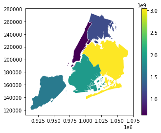
GeoPandas还可以绘制地图,所以我们可以检查几何图形在太空中的显示方式。若要绘制活动几何图形,请调用 GeoDataFrame.plot() 。要按另一列进行颜色编码,请将该列作为第一个参数传入。在下面的示例中,我们绘制激活的几何图形列和颜色代码 "area" 纵队。我们也想展示一个传奇 (legend=True )。
[9]:
gdf.plot("area", legend=True)
[9]:
<AxesSubplot:>
您还可以使用以交互方式浏览数据 GeoDataFrame.explore() ,它的行为方式与 plot() 而是返回交互式地图。
[10]:
gdf.explore("area", legend=False)
---------------------------------------------------------------------------
ModuleNotFoundError                       Traceback (most recent call last)
File /usr/local/lib/python3.10/dist-packages/geopandas-0.10.2+79.g3abc6a7-py3.10.egg/geopandas/explore.py:271, in _explore(df, column, cmap, color, m, tiles, attr, tooltip, popup, highlight, categorical, legend, scheme, k, vmin, vmax, width, height, categories, classification_kwds, control_scale, marker_type, marker_kwds, style_kwds, highlight_kwds, missing_kwds, tooltip_kwds, popup_kwds, legend_kwds, map_kwds, **kwargs)
    270     import matplotlib.pyplot as plt
--> 271     from mapclassify import classify
    272 except (ImportError, ModuleNotFoundError):

ModuleNotFoundError: No module named 'mapclassify'

During handling of the above exception, another exception occurred:

ImportError                               Traceback (most recent call last)
Input In [10], in <cell line: 1>()
----> 1 gdf.explore("area", legend=False)

File /usr/local/lib/python3.10/dist-packages/geopandas-0.10.2+79.g3abc6a7-py3.10.egg/geopandas/geodataframe.py:1903, in GeoDataFrame.explore(self, *args, **kwargs)
   1900 @doc(_explore)
   1901 def explore(self, *args, **kwargs):
   1902     """Interactive map based on folium/leaflet.js"""
-> 1903     return _explore(self, *args, **kwargs)

File /usr/local/lib/python3.10/dist-packages/geopandas-0.10.2+79.g3abc6a7-py3.10.egg/geopandas/explore.py:273, in _explore(df, column, cmap, color, m, tiles, attr, tooltip, popup, highlight, categorical, legend, scheme, k, vmin, vmax, width, height, categories, classification_kwds, control_scale, marker_type, marker_kwds, style_kwds, highlight_kwds, missing_kwds, tooltip_kwds, popup_kwds, legend_kwds, map_kwds, **kwargs)
    271     from mapclassify import classify
    272 except (ImportError, ModuleNotFoundError):
--> 273     raise ImportError(
    274         "The 'folium', 'matplotlib' and 'mapclassify' packages are required for "
    275         "'explore()'. You can install them using "
    276         "'conda install -c conda-forge folium matplotlib mapclassify' "
    277         "or 'pip install folium matplotlib mapclassify'."
    278     )
    280 # xyservices is an optional dependency
    281 try:

ImportError: The 'folium', 'matplotlib' and 'mapclassify' packages are required for 'explore()'. You can install them using 'conda install -c conda-forge folium matplotlib mapclassify' or 'pip install folium matplotlib mapclassify'.
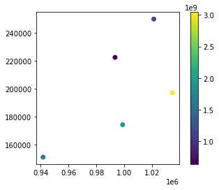
切换激活的几何体 (GeoDataFrame.set_geometry )到质心,我们可以使用点几何绘制相同的数据。
[11]:
gdf = gdf.set_geometry("centroid")
gdf.plot("area", legend=True)
[11]:
<AxesSubplot:>
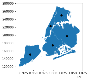
我们还可以将这两个层次 GeoSeries 在彼此的顶端。我们只需要使用一个地块作为另一个地块的轴。
[12]:
ax = gdf["geometry"].plot()
gdf["centroid"].plot(ax=ax, color="black")
[12]:
<AxesSubplot:>
现在,我们将活动几何图形设置回原始状态 GeoSeries 。
[13]:
gdf = gdf.set_geometry("geometry")
用户指南
请参阅更多信息 mapping in the User Guide 。
几何图形创建#
我们可以进一步处理几何体,并在已有的基础上创建新的形状。
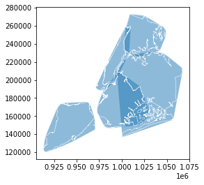
凸壳#
如果我们对面的凸包感兴趣,我们可以访问 GeoDataFrame.convex_hull 。
[14]:
gdf["convex_hull"] = gdf.convex_hull
[15]:
ax = gdf["convex_hull"].plot(alpha=.5)  # saving the first plot as an axis and setting alpha (transparency) to 0.5
gdf["boundary"].plot(ax=ax, color="white", linewidth=.5)  # passing the first plot and setting linewitdth to 0.5
[15]:
<AxesSubplot:>
缓冲层#
在其他情况下,我们可能需要使用缓冲几何 GeoDataFrame.buffer() 。几何方法会自动应用于活动几何,但我们可以将它们直接应用于任何 GeoSeries 也是。让我们缓冲这些行政区和它们的质心,并在彼此的顶部进行绘制。
[16]:
# buffering the active geometry by 10 000 feet (geometry is already in feet)
gdf["buffered"] = gdf.buffer(10000)

# buffering the centroid geometry by 10 000 feet (geometry is already in feet)
gdf["buffered_centroid"] = gdf["centroid"].buffer(10000)
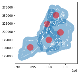
[17]:
ax = gdf["buffered"].plot(alpha=.5)  # saving the first plot as an axis and setting alpha (transparency) to 0.5
gdf["buffered_centroid"].plot(ax=ax, color="red", alpha=.5)  # passing the first plot as an axis to the second
gdf["boundary"].plot(ax=ax, color="white", linewidth=.5)  # passing the first plot and setting linewitdth to 0.5
[17]:
<AxesSubplot:>
用户指南
请参阅更多信息 geometry creation and manipulation in the User Guide 。
几何关系#
我们还可以询问不同几何图形的空间关系。使用上面的几何图形,我们可以检查哪些缓冲的行政区与布鲁克林的原始几何图形相交,即距离布鲁克林不到10,000英尺。
首先,我们得到布鲁克林的一个多边形。
[18]:
brooklyn = gdf.loc["Brooklyn", "geometry"]
brooklyn
[18]:

该多边形是一个 shapely geometry object ,与GeoPandas中使用的任何其他几何体一样。
[19]:
type(brooklyn)
[19]:
shapely.geometry.multipolygon.MultiPolygon
然后我们可以检查其中的哪些几何图形 gdf["buffered"] 与其相交。
[20]:
gdf["buffered"].intersects(brooklyn)
[20]:
BoroName
Staten Island     True
Queens            True
Brooklyn          True
Manhattan         True
Bronx            False
dtype: bool
只有布朗克斯(北部)距离布鲁克林超过10000英尺。所有其他的都更近,并与我们的多边形相交。
或者,我们可以检查哪些缓冲质心完全在原始行政区的多边形内。在这种情况下,两者都 GeoSeries 对齐,并对每行执行检查。
[21]:
gdf["within"] = gdf["buffered_centroid"].within(gdf)
gdf["within"]
[21]:
BoroName
Staten Island     True
Queens            True
Brooklyn         False
Manhattan        False
Bronx            False
Name: within, dtype: bool
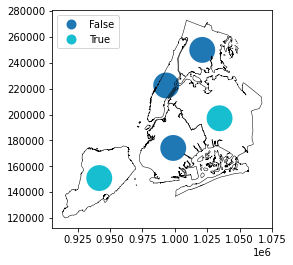
我们可以把结果画在地图上,以确认这一发现。
[22]:
gdf = gdf.set_geometry("buffered_centroid")
ax = gdf.plot("within", legend=True, categorical=True, legend_kwds={'loc': "upper left"})  # using categorical plot and setting the position of the legend
gdf["boundary"].plot(ax=ax, color="black", linewidth=.5)  # passing the first plot and setting linewitdth to 0.5
[22]:
<AxesSubplot:>
推算#
每个人 GeoSeries 其坐标参考系(CRS)可在 GeoSeries.crs 。CRS会告诉GeoPandas这些几何图形的坐标在地球表面的位置。在某些情况下,CRS是地理上的,这意味着坐标在纬度和经度上。在这些情况下,其CRS是WGS84,具有授权代码 EPSG:4326 。让我们看看我们纽约各区的投影 GeoDataFrame 。
[23]:
gdf.crs
[23]:
<Derived Projected CRS: EPSG:2263>
Name: NAD83 / New York Long Island (ftUS)
Axis Info [cartesian]:
- X[east]: Easting (US survey foot)
- Y[north]: Northing (US survey foot)
Area of Use:
- name: United States (USA) - New York - counties of Bronx; Kings; Nassau; New York; Queens; Richmond; Suffolk.
- bounds: (-74.26, 40.47, -71.8, 41.3)
Coordinate Operation:
- name: SPCS83 New York Long Island zone (US Survey feet)
- method: Lambert Conic Conformal (2SP)
Datum: North American Datum 1983
- Ellipsoid: GRS 1980
- Prime Meridian: Greenwich
几何图形已加入 EPSG:2263 以英尺为单位的坐标。我们可以很容易地重新投射一个 GeoSeries 到另一个CRS,比如 EPSG:4326 使用 GeoSeries.to_crs() 。
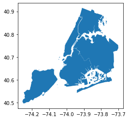
[24]:
gdf = gdf.set_geometry("geometry")
boroughs_4326 = gdf.to_crs("EPSG:4326")
boroughs_4326.plot()
[24]:
<AxesSubplot:>
[25]:
boroughs_4326.crs
[25]:
<Geographic 2D CRS: EPSG:4326>
Name: WGS 84
Axis Info [ellipsoidal]:
- Lat[north]: Geodetic latitude (degree)
- Lon[east]: Geodetic longitude (degree)
Area of Use:
- name: World.
- bounds: (-180.0, -90.0, 180.0, 90.0)
Datum: World Geodetic System 1984 ensemble
- Ellipsoid: WGS 84
- Prime Meridian: Greenwich
请注意沿曲线图轴线的坐标差异。以前我们有12万到28万英尺,现在我们有40.5到40.9度。在这种情况下, boroughs_4326 有一个 "geometry" WGS84中的列,但其他所有列(带有质心等)保留在原始的CRS中。
警告
对于依赖于距离或面积的操作,您始终需要使用投影CRS(以米、英尺、公里等为单位)不是地理上的(以度计)。GeoPandas的操作是平面的,而度数反映了球体上的位置。因此,使用度的空间运算可能不会产生正确的结果。例如,结果为 gdf.area.sum() (预计CRS)为8 429 911 572 ft2,但结果为 boroughs_4326.area.sum() (地理CRS)为0.083。
用户指南
请参阅更多信息 projections in the User Guide 。
接下来是什么?#
有了GeoPandas,我们可以做的比目前为止引入的要多得多,从 aggregations ,至 spatial joins ,至 geocoding ,以及 much more 。
去那边的 User Guide 要了解有关GeoPandas的不同功能的更多信息,请参阅 Examples 查看如何使用它们,或者到 API reference 了解详情。