备注
来自PYSAL的用于GeoPandas的Clopeth分类方案#
 PySAL is a Spatial Analysis Library <>, which packages fast spatial algorithms used in various fields. These include Exploratory spatial data analysis, spatial inequality analysis, spatial analysis on networks, spatial dynamics, and many more.
当使用一组颜色绘制测量时,它在地貌熊猫的引擎盖下使用。有许多方法可以将数据分类到不同的箱中,具体取决于许多分类方案。
例如,如果我们有20个国家/地区的年平均气温在5摄氏度到25摄氏度之间,我们可以按以下方式将它们分类到4个箱子中:* Quantiles - Separates the rows into equal parts, 5 countries per bin. * 相等间隔-将测量间隔等分成等份,每箱5C。*自然中断(Fischer Jenks)-此算法尝试将行拆分成自然出现的集群。每个面元的数字将取决于观测值在间隔上的位置。
[1]:
import geopandas as gpd
import matplotlib.pyplot as plt
[2]:
# We use a PySAL example shapefile
import libpysal as ps

pth = ps.examples.get_path("columbus.shp")
tracts = gpd.GeoDataFrame.from_file(pth)
print('Observations, Attributes:',tracts.shape)
tracts.head()
Observations, Attributes: (49, 21)
[2]:
| AREA | PERIMETER | COLUMBUS_ | COLUMBUS_I | POLYID | NEIG | HOVAL | INC | CRIME | OPEN | ... | DISCBD | X | Y | NSA | NSB | EW | CP | THOUS | NEIGNO | geometry | |
|---|---|---|---|---|---|---|---|---|---|---|---|---|---|---|---|---|---|---|---|---|---|
| 0 | 0.309441 | 2.440629 | 2 | 5 | 1 | 5 | 80.467003 | 19.531 | 15.725980 | 2.850747 | ... | 5.03 | 38.799999 | 44.070000 | 1.0 | 1.0 | 1.0 | 0.0 | 1000.0 | 1005.0 | POLYGON ((8.62413 14.23698, 8.55970 14.74245, ... |
| 1 | 0.259329 | 2.236939 | 3 | 1 | 2 | 1 | 44.567001 | 21.232 | 18.801754 | 5.296720 | ... | 4.27 | 35.619999 | 42.380001 | 1.0 | 1.0 | 0.0 | 0.0 | 1000.0 | 1001.0 | POLYGON ((8.25279 14.23694, 8.28276 14.22994, ... |
| 2 | 0.192468 | 2.187547 | 4 | 6 | 3 | 6 | 26.350000 | 15.956 | 30.626781 | 4.534649 | ... | 3.89 | 39.820000 | 41.180000 | 1.0 | 1.0 | 1.0 | 0.0 | 1000.0 | 1006.0 | POLYGON ((8.65331 14.00809, 8.81814 14.00205, ... |
| 3 | 0.083841 | 1.427635 | 5 | 2 | 4 | 2 | 33.200001 | 4.477 | 32.387760 | 0.394427 | ... | 3.70 | 36.500000 | 40.520000 | 1.0 | 1.0 | 0.0 | 0.0 | 1000.0 | 1002.0 | POLYGON ((8.45950 13.82035, 8.47341 13.83227, ... |
| 4 | 0.488888 | 2.997133 | 6 | 7 | 5 | 7 | 23.225000 | 11.252 | 50.731510 | 0.405664 | ... | 2.83 | 40.009998 | 38.000000 | 1.0 | 1.0 | 1.0 | 0.0 | 1000.0 | 1007.0 | POLYGON ((8.68527 13.63952, 8.67758 13.72221, ... |
5 rows × 21 columns
谋划犯罪变量#
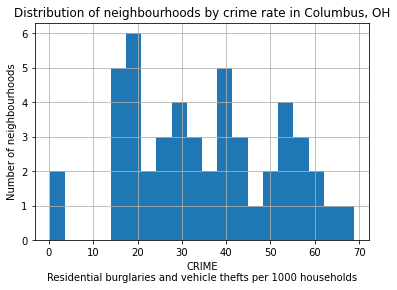
在本例中,我们将查看俄亥俄州哥伦布市的邻居级统计数据。我们想知道犯罪率变量是如何在城市中分布的。
从 shapefile’s metadata :>CRIME :住宅入室盗窃和车辆盗窃每1000户家庭
[3]:
# Let's take a look at how the CRIME variable is distributed with a histogram
tracts['CRIME'].hist(bins=20)
plt.xlabel('CRIME\nResidential burglaries and vehicle thefts per 1000 households')
plt.ylabel('Number of neighbourhoods')
plt.title('Distribution of neighbourhoods by crime rate in Columbus, OH')
plt.show()
现在让我们看看没有分类方案是什么样子:
[4]:
tracts.plot(column='CRIME', cmap='OrRd', edgecolor='k', legend=True)
[4]:
<AxesSubplot:>
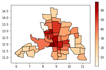
所有49个街区都是沿着从白到暗红色的渐变上色的,但人眼很难比较彼此相距较远的形状的颜色。在这种情况下,特别难对米色的外围地区进行排名。
取而代之的是,我们将它们分类到颜色箱中。
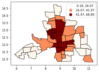
按分位数分类#
分位数将创建吸引人的地图,在每个类别中放置相同数量的观测:如果您有30个县和6个数据类别,则每个类别中将有5个县。分位数的问题是,您最终得到的类可能具有非常不同的数字范围(例如,1-4、4-9、9-250)。
[5]:
# Splitting the data in three shows some spatial clustering around the center
tracts.plot(column='CRIME', scheme='quantiles', k=3, cmap='OrRd', edgecolor='k', legend=True)
[5]:
<AxesSubplot:>
[6]:
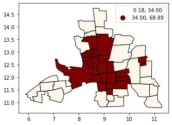
# We can also see where the top and bottom halves are located
tracts.plot(column='CRIME', scheme='quantiles', k=2, cmap='OrRd', edgecolor='k', legend=True)
[6]:
<AxesSubplot:>
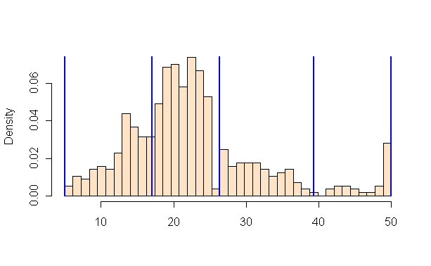
等间隔分类#
相等间隔将数据分为相等大小的类别(例如,0-10、10-20、20-30等)。并且在通常分布在整个范围内的数据上效果最好。注意:如果您的数据偏向一端,或者如果您有一个或两个非常大的离群值,请避免使用相等间隔。
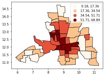
[7]:
tracts.plot(column='CRIME', scheme='equal_interval', k=4, cmap='OrRd', edgecolor='k', legend=True)
[7]:
<AxesSubplot:>
[8]:
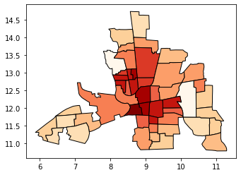
# No legend here as we'd be out of space
tracts.plot(column='CRIME', scheme='equal_interval', k=12, cmap='OrRd', edgecolor='k')
[8]:
<AxesSubplot:>
按自然间歇进行分类#
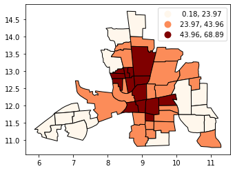
自然间歇期是一种“最佳”分类方案,它找到的分类间隔期将最小化类内差异和最大化类间差异。这种方法的一个缺点是每个数据集生成唯一的分类解决方案,并且如果您需要跨地图进行比较,例如在地图集或系列中(例如,1980、1990、2000各有一个地图),您可能希望使用可应用于所有地图的单个方案。
[9]:
# Compare this to the previous 3-bin figure with quantiles
tracts.plot(column='CRIME', scheme='natural_breaks', k=3, cmap='OrRd', edgecolor='k', legend=True)
[9]:
<AxesSubplot:>
PYSAL中的其他分类方案#
Geopandas只包括在PYSAL中发现的最常用的量词。为了使用其他列,您需要将它们作为附加列添加到GeoDataFrame中。
Max-p算法基于一组区域、每个区域上的属性矩阵和楼层约束来内生地确定区域的数量(P)。下限约束定义了每个地区变量必须达到的最小范围;例如,约束可能是每个地区必须拥有的最小人口。Max-p进一步对区域内的区域实施邻接约束。
[10]:
def max_p(values, k):
    """
    Given a list of values and `k` bins,
    returns a list of their Maximum P bin number.
    """
    from mapclassify import MaxP
    binning = MaxP(values, k=k)
    return binning.yb

tracts['Max_P'] = max_p(tracts['CRIME'].values, k=5)
tracts.head()
[10]:
| AREA | PERIMETER | COLUMBUS_ | COLUMBUS_I | POLYID | NEIG | HOVAL | INC | CRIME | OPEN | ... | X | Y | NSA | NSB | EW | CP | THOUS | NEIGNO | geometry | Max_P | |
|---|---|---|---|---|---|---|---|---|---|---|---|---|---|---|---|---|---|---|---|---|---|
| 0 | 0.309441 | 2.440629 | 2 | 5 | 1 | 5 | 80.467003 | 19.531 | 15.725980 | 2.850747 | ... | 38.799999 | 44.070000 | 1.0 | 1.0 | 1.0 | 0.0 | 1000.0 | 1005.0 | POLYGON ((8.62413 14.23698, 8.55970 14.74245, ... | 0 |
| 1 | 0.259329 | 2.236939 | 3 | 1 | 2 | 1 | 44.567001 | 21.232 | 18.801754 | 5.296720 | ... | 35.619999 | 42.380001 | 1.0 | 1.0 | 0.0 | 0.0 | 1000.0 | 1001.0 | POLYGON ((8.25279 14.23694, 8.28276 14.22994, ... | 0 |
| 2 | 0.192468 | 2.187547 | 4 | 6 | 3 | 6 | 26.350000 | 15.956 | 30.626781 | 4.534649 | ... | 39.820000 | 41.180000 | 1.0 | 1.0 | 1.0 | 0.0 | 1000.0 | 1006.0 | POLYGON ((8.65331 14.00809, 8.81814 14.00205, ... | 2 |
| 3 | 0.083841 | 1.427635 | 5 | 2 | 4 | 2 | 33.200001 | 4.477 | 32.387760 | 0.394427 | ... | 36.500000 | 40.520000 | 1.0 | 1.0 | 0.0 | 0.0 | 1000.0 | 1002.0 | POLYGON ((8.45950 13.82035, 8.47341 13.83227, ... | 2 |
| 4 | 0.488888 | 2.997133 | 6 | 7 | 5 | 7 | 23.225000 | 11.252 | 50.731510 | 0.405664 | ... | 40.009998 | 38.000000 | 1.0 | 1.0 | 1.0 | 0.0 | 1000.0 | 1007.0 | POLYGON ((8.68527 13.63952, 8.67758 13.72221, ... | 3 |
5 rows × 22 columns
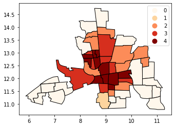
[11]:
tracts.plot(column='Max_P', cmap='OrRd', edgecolor='k', categorical=True, legend=True)
[11]:
<AxesSubplot:>
[ ]: