非线性求解器
这是一个通用非线性多维解算器的集合。这些求解者发现 x 为此, F(x) = 0 。两者都有 x 和 F 可以是多维的。
例行公事
大型非线性解算器:
|
求函数的根,对逆雅可比矩阵使用Krylov近似。 |
|
使用(扩展的)安德森混合求函数的根。 |
一般非线性解算器:
|
使用Broyden的第一雅可比近似求函数的根。 |
|
使用Broyden的二次雅可比近似求函数的根。 |
简单迭代:
|
使用调谐的对角雅可比近似求函数的根。 |
|
使用标量雅可比近似求函数的根。 |
|
使用对角Broyden Jacobian近似求函数的根。 |
示例
小问题
>>> def F(x):
...    return np.cos(x) + x[::-1] - [1, 2, 3, 4]
>>> import scipy.optimize
>>> x = scipy.optimize.broyden1(F, [1,1,1,1], f_tol=1e-14)
>>> x
array([ 4.04674914,  3.91158389,  2.71791677,  1.61756251])
>>> np.cos(x) + x[::-1]
array([ 1.,  2.,  3.,  4.])
大问题
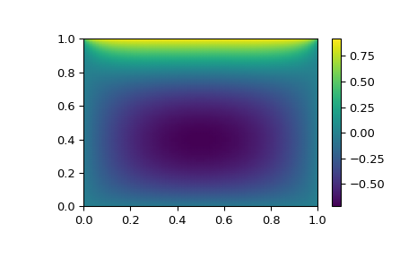
假设我们需要在正方形上解下面的积分微分方程 \([0,1]\times[0,1]\) :
\[\nabla^2 P=10\Left(\int_0^1\int_0^1\cosh(P)\,dx\,dy\right)^2\]
使用 \(P(x,1) = 1\) 和 \(P=0\) 在广场边界的其他地方。
解决方案可以使用 newton_krylov 解算器:
import numpy as np
from scipy.optimize import newton_krylov
from numpy import cosh, zeros_like, mgrid, zeros

# parameters
nx, ny = 75, 75
hx, hy = 1./(nx-1), 1./(ny-1)

P_left, P_right = 0, 0
P_top, P_bottom = 1, 0

def residual(P):
    d2x = zeros_like(P)
    d2y = zeros_like(P)

    d2x[1:-1] = (P[2:]   - 2*P[1:-1] + P[:-2]) / hx/hx
    d2x[0]    = (P[1]    - 2*P[0]    + P_left)/hx/hx
    d2x[-1]   = (P_right - 2*P[-1]   + P[-2])/hx/hx

    d2y[:,1:-1] = (P[:,2:] - 2*P[:,1:-1] + P[:,:-2])/hy/hy
    d2y[:,0]    = (P[:,1]  - 2*P[:,0]    + P_bottom)/hy/hy
    d2y[:,-1]   = (P_top   - 2*P[:,-1]   + P[:,-2])/hy/hy

    return d2x + d2y - 10*cosh(P).mean()**2

# solve
guess = zeros((nx, ny), float)
sol = newton_krylov(residual, guess, method='lgmres', verbose=1)
print('Residual: %g' % abs(residual(sol)).max())

# visualize
import matplotlib.pyplot as plt
x, y = mgrid[0:1:(nx*1j), 0:1:(ny*1j)]
plt.pcolormesh(x, y, sol, shading='gouraud')
plt.colorbar()
plt.show()