scipy.special.eval_legendre
- scipy.special.eval_legendre(n, x, out=None) = <ufunc 'eval_legendre'>
在一点计算勒让德多项式。
勒让德多项式可以通过高斯超几何函数来定义 \({{}}_2F_1\) 作为
\[Pn(X)={}2F1(-n,n+1;1;(1-x)/2)。\]什么时候 \(n\) 是整数,则结果是一次多项式 \(n\) 。请参见22.5.49中的 [AS] 有关详细信息,请参阅。
- 参数
- narray_like
多项式的次数。如果不是整数,则通过与高斯超几何函数的关系确定结果。
- xarray_like
勒让德多项式的求值点
- 退货
- Pndarray
勒让德多项式的取值
参见
roots_legendre勒让德多项式的根和求积权
legendre勒让德多项式对象
hyp2f1高斯超几何函数
numpy.polynomial.legendre.Legendre勒让德系列
参考文献
- AS
米尔顿·阿布拉莫维茨和艾琳·A·斯特根主编。包含公式、图表和数学表的数学函数手册。纽约:多佛,1972年。
示例
>>> from scipy.special import eval_legendre
求x=0的零阶勒让德多项式
>>> eval_legendre(0, 0)
1.0
求-1到1之间的一阶勒让德多项式
>>> X = np.linspace(-1, 1, 5)  # Domain of Legendre polynomials
>>> eval_legendre(1, X)
array([-1. , -0.5,  0. ,  0.5,  1. ])
求x=0时0到4阶的勒让德多项式
>>> N = range(0, 5)
>>> eval_legendre(N, 0)
array([ 1.   ,  0.   , -0.5  ,  0.   ,  0.375])
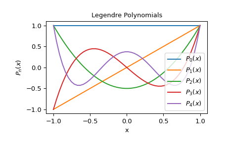
绘制0到4阶Legendre多项式
>>> X = np.linspace(-1, 1)
>>> import matplotlib.pyplot as plt
>>> for n in range(0, 5):
...     y = eval_legendre(n, X)
...     plt.plot(X, y, label=r'$P_{}(x)$'.format(n))
>>> plt.title("Legendre Polynomials")
>>> plt.xlabel("x")
>>> plt.ylabel(r'$P_n(x)$')
>>> plt.legend(loc='lower right')
>>> plt.show()