计算能力
Computes the GC-bias using Benjamini's method [Benjamini & Speed (2012). Nucleic Acids Research, 40(10). doi: 10.1093/nar/gks001]. The GC-bias is visualized and the resulting table can be used tocorrect the bias with correctGCBias.
usage: computeGCBias -b file.bam --effectiveGenomeSize 2150570000 -g mm9.2bit -l 200 --GCbiasFrequenciesFile freq.txt
help: computeGCBias -h / computeGCBias --help
Required arguments
- --bamfile, -b
Sorted BAM file.
- --effectiveGenomeSize
The effective genome size is the portion of the genome that is mappable. Large fractions of the genome are stretches of NNNN that should be discarded. Also, if repetitive regions were not included in the mapping of reads, the effective genome size needs to be adjusted accordingly. A table of values is available here: http://deeptools.readthedocs.io/en/latest/content/feature/effectiveGenomeSize.html .
- --genome, -g
Genome in two bit format. Most genomes can be found here: http://hgdownload.cse.ucsc.edu/gbdb/ Search for the .2bit ending. Otherwise, fasta files can be converted to 2bit using the UCSC programm called faToTwoBit available for different plattforms at http://hgdownload.cse.ucsc.edu/admin/exe/
- --GCbiasFrequenciesFile, -freq, -o
Path to save the file containing the observed and expected read frequencies per %GC-content. This file is needed to run the correctGCBias tool. This is a text file.
Optional arguments
- --fragmentLength, -l
Fragment length used for the sequencing. If paired-end reads are used, the fragment length is computed based from the bam file
- --sampleSize
Number of sampling points to be considered. (Default: 50000000.0)
- --extraSampling
BED file containing genomic regions for which extra sampling is required because they are underrepresented in the genome.
- --version
show program's version number and exit
- --region, -r
Region of the genome to limit the operation to - this is useful when testing parameters to reduce the computing time. The format is chr:start:end, for example --region chr10 or --region chr10:456700:891000.
- --blackListFileName, -bl
A BED or GTF file containing regions that should be excluded from all analyses. Currently this works by rejecting genomic chunks that happen to overlap an entry. Consequently, for BAM files, if a read partially overlaps a blacklisted region or a fragment spans over it, then the read/fragment might still be considered. Please note that you should adjust the effective genome size, if relevant.
- --numberOfProcessors, -p
Number of processors to use. Type "max/2" to use half the maximum number of processors or "max" to use all available processors. (Default: 1)
- --verbose, -v
Set to see processing messages.
Diagnostic plot options
- --biasPlot
If given, a diagnostic image summarizing the GC-bias will be saved.
- --plotFileFormat
Possible choices: png, pdf, svg, eps, plotly
image format type. If given, this option overrides the image format based on the plotFile ending. The available options are: "png", "eps", "pdf", "plotly" and "svg"
- --regionSize
To plot the reads per %GC over a regionthe size of the region is required. By default, the bin size is set to 300 bases, which is close to the standard fragment size for Illumina machines. However, if the depth of sequencing is low, a larger bin size will be required, otherwise many bins will not overlap with any read (Default: 300)
背景
computeGCBias 是根据一篇论文 Benjamini and Speed . GC偏差诊断的基本假设是,理想样本应显示整个基因组的序列读取的均匀分布,即基因组的所有区域应具有相似的读取次数,而不管其碱基对组成如何。实际上,在测序方案的文库准备过程中,用于基于PCR的扩增的DNA聚合酶更倾向于GC富集区。这将影响测序结果,因为由于DNA聚合酶的偏好,对富含GC的区域有更多的读取。
computeGCbias 将首先计算 预期的GC配置文件 通过计算每个GC片段的固定大小的DNA片段数量,其中GC片段被定义为给定长度的基因组区域中G或C的数量。结果基本上是一个柱状图,描绘了每种类型基因组区域的DNA片段频率,gc分数介于0%到100%之间。这对于每个参考基因组都是不同的,但与实际的测序实验无关。
然后将预期的DNA片段分布与 观察到的GC曲线 ,通过计算每个GC部分的顺序读取数生成。
在一个理想的实验中,所观察到的GC剖面,当然,看起来像预期的剖面。申请时确实如此 computeGCBias 模拟读取。
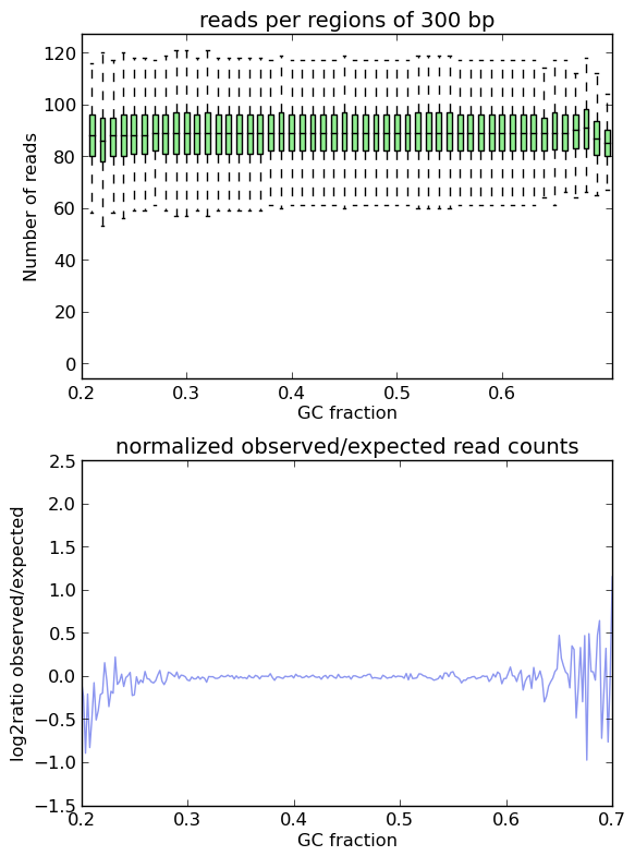
如您所见,两个图都基于 模拟读取 不要显示特定GC内容物箱的富集或耗尽,在log2radio周围有一条几乎平坦的线,0(=比率(观察/预期)为1)。X轴两端的波动是由于只有极少数区域 果蝇属 基因组具有如此极端的GC片段,因此随机取样中提取的片段数量可能会有所不同。
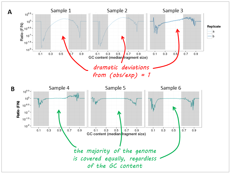
现在,让我们看看 real-life data 来自基因组DNA测序。图A和图B可以清楚地区分,图中实验之间发生的主要变化是,图A中的样品用过多的PCR循环和标准聚合酶制备,而图B中的样品只需进行很少的扩增。使用高保真DNA聚合酶进行聚合。
备注
由于不同生物的GC含量差异很大,因此预期的GC图谱取决于参考基因组。例如,在小鼠样本中(小鼠基因组的平均GC含量:45%)的GC片段比来自,例如, 恶性疟原虫 (平均基因组GC含量 恶性疟原虫 :20%)。
从读取分布计算中排除区域
在某些情况下,从读取分布的计算中排除某些区域是有意义的,以提高计算的准确性。有几种区域不希望显示与背景匹配的读分布,或者参考基因组的不确定性可能太大。请考虑以下几点:
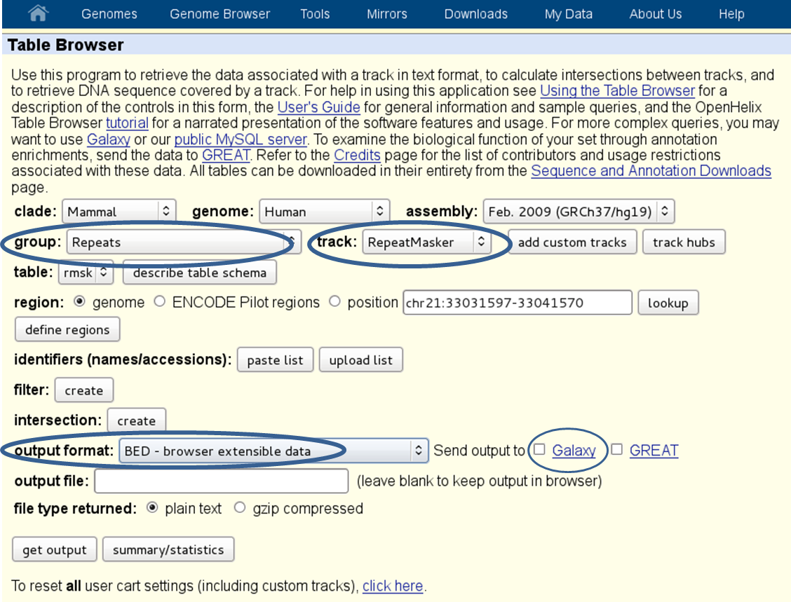
重复区域 :如果多重读取(读取多个基因组位置的映射)被排除在 [BAM] []文件,它将有助于排除已知的重复区域。您可以从中获取已知重复区域的床位文件 UCSC Table Browser (有关人类重复元素的示例,请参见下面的屏幕截图)。
低可映射性区域 :这些区域中的读取映射出了众所周知的失败,我们建议从GC计算中排除具有可映射性问题的已知区域。您可以从UCSC下载不同读取长度的可映射性跟踪,例如 mouse 和 human . 在github deeptools文件夹“scripts”中,可以找到一个名为
mappabilityBigWig_to_unmappableBed.sh它将使 [大人物] []从UCSC映射到BED文件的可映射性文件。ChIP-seq peaks :在Chip Seq样本中 预期 某些地区 应该 根据背景分布显示比预期更多的读取,因此从GC偏差计算中排除这些区域是绝对有意义的。我们建议运行一个简单的、非保守的峰值,调用未更正的 [BAM] []首先归档以获取峰值区域的bed文件,然后将其提供给
computeGCbias.
使用实例
$ computeGCBias -b H3K27Me3.bam --effectiveGenomeSize 2695000000
   --genome genome.2bit -l 200 -freq freq_test.txt
   --region X --biasPlot test_gc.png
deepTools Galaxy <http://deeptools.ie-freiburg.mpg.de> _. |
code @ github <https://github.com/deeptools/deepTools/> _. |