scipy.stats.binned_statistic
- scipy.stats.binned_statistic(x, values, statistic='mean', bins=10, range=None)[源代码]
计算一组或多组数据的入库统计信息。
这是直方图函数的推广。直方图将空间划分为存储箱,并返回每个存储箱中点数的计数。此函数允许计算每个面元内的值(或值集)的总和、平均值、中位数或其他统计信息。
- 参数
- x(n,)类似数组
要入库的值序列。
- values(N,)ARRAY_LIKE或(N,)ARRAY_LIKE列表
将计算统计数据的数据。此形状必须与 x ,或一组序列-每个序列的形状与 x 。如果 values 是一组序列,则将对每个序列单独计算统计信息。
- statistic字符串或可调用,可选
要计算的统计数据(默认值为“Mean”)。以下统计数据可用:
“Mean”:计算每个面元内各点的平均值。空垃圾箱将由NaN代表。
‘std’:计算每个仓位内的标准偏差。这是在ddof=0时隐式计算的。
“中位数”:计算每个垃圾箱内各点的值的中位数。空垃圾箱将由NaN代表。
‘count’:计算每个bin内的点数。这与未加权的直方图相同。 values 未引用数组。
‘sum’:计算每个bin内的点的值之和。这与加权直方图相同。
‘min’:计算每个bin内的点的最小值。空垃圾箱将由NaN代表。
‘max’:计算每个bin内的点的最大值。空垃圾箱将由NaN代表。
函数:一个用户定义的函数,它接受一维的值数组,并输出单个数值统计数据。将对每个bin中的值调用此函数。空箱将由函数([])表示,如果返回错误,则用NaN表示。
- bins整型或标量序列,可选
如果 bins 是一个整数,它定义给定范围内的等宽箱数(默认为10)。如果 bins 是一个序列,它定义了仓位边缘,包括最右边的边缘,从而允许非均匀仓位宽度。中的值 x 将小于最低条柱边缘的值指定给条柱编号0,将超出最高条柱边缘的值指定给
bins[-1]。如果指定了仓边,则仓数将为(nx=len(仓位)-1)。- range(浮点型,浮点型)或 [(浮点数,浮点数)] ,可选
垃圾箱的下限范围和上限范围。如果未提供,则范围仅为
(x.min(), x.max())。范围之外的值将被忽略。
- 退货
- statistic阵列
每个箱中选定统计信息的值。
- bin_edges数据类型浮点数组
退回仓边
(length(statistic)+1)。- 二进制数:整数的一维ndarray
料箱的索引(对应于 bin_edges ),其中每个值 x 属于这里。长度与相同 values 。二进制数 i 表示相应的值在(Bin_Edges)之间 [i-1] ,bin_edge [i] )。
注意事项
除了最后一个(最右边的)垃圾箱外,所有的垃圾箱都是半开的。换句话说,如果 bins 是
[1, 2, 3, 4],那么第一个垃圾箱是[1, 2)(包括1个,但不包括2个)和第二个[2, 3)。然而,最后一个垃圾箱是[3, 4],其中 包括 4.0.11.0 新版功能.
示例
>>> from scipy import stats
>>> import matplotlib.pyplot as plt
先举几个基本的例子:
在给定样本的范围内创建两个等间距的箱,并对每个箱中的相应值求和:
>>> values = [1.0, 1.0, 2.0, 1.5, 3.0]
>>> stats.binned_statistic([1, 1, 2, 5, 7], values, 'sum', bins=2)
BinnedStatisticResult(statistic=array([4. , 4.5]),
        bin_edges=array([1., 4., 7.]), binnumber=array([1, 1, 1, 2, 2]))
还可以传递多个值数组。统计数据在每个集合上独立计算:
>>> values = [[1.0, 1.0, 2.0, 1.5, 3.0], [2.0, 2.0, 4.0, 3.0, 6.0]]
>>> stats.binned_statistic([1, 1, 2, 5, 7], values, 'sum', bins=2)
BinnedStatisticResult(statistic=array([[4. , 4.5],
       [8. , 9. ]]), bin_edges=array([1., 4., 7.]),
       binnumber=array([1, 1, 1, 2, 2]))
>>> stats.binned_statistic([1, 2, 1, 2, 4], np.arange(5), statistic='mean',
...                        bins=3)
BinnedStatisticResult(statistic=array([1., 2., 4.]),
        bin_edges=array([1., 2., 3., 4.]),
        binnumber=array([1, 2, 1, 2, 3]))
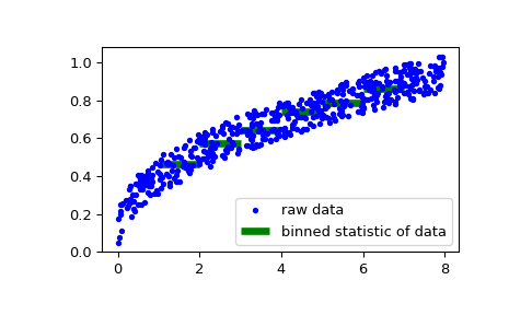
作为第二个示例,我们现在生成一些作为风速函数的帆船速度的随机数据,然后确定我们的船在特定风速下的速度:
>>> rng = np.random.default_rng()
>>> windspeed = 8 * rng.random(500)
>>> boatspeed = .3 * windspeed**.5 + .2 * rng.random(500)
>>> bin_means, bin_edges, binnumber = stats.binned_statistic(windspeed,
...                 boatspeed, statistic='median', bins=[1,2,3,4,5,6,7])
>>> plt.figure()
>>> plt.plot(windspeed, boatspeed, 'b.', label='raw data')
>>> plt.hlines(bin_means, bin_edges[:-1], bin_edges[1:], colors='g', lw=5,
...            label='binned statistic of data')
>>> plt.legend()
现在我们可以使用
binnumber要选择风速低于1的所有数据点,请执行以下操作:>>> low_boatspeed = boatspeed[binnumber == 0]
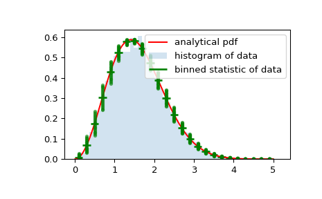
作为最后一个示例,我们将使用
bin_edges和binnumber要在规则直方图和概率分布函数的顶部绘制显示每箱平均值周围的平均值和分布的分布图,请执行以下操作:>>> x = np.linspace(0, 5, num=500) >>> x_pdf = stats.maxwell.pdf(x) >>> samples = stats.maxwell.rvs(size=10000)
>>> bin_means, bin_edges, binnumber = stats.binned_statistic(x, x_pdf,
...         statistic='mean', bins=25)
>>> bin_width = (bin_edges[1] - bin_edges[0])
>>> bin_centers = bin_edges[1:] - bin_width/2
>>> plt.figure()
>>> plt.hist(samples, bins=50, density=True, histtype='stepfilled',
...          alpha=0.2, label='histogram of data')
>>> plt.plot(x, x_pdf, 'r-', label='analytical pdf')
>>> plt.hlines(bin_means, bin_edges[:-1], bin_edges[1:], colors='g', lw=2,
...            label='binned statistic of data')
>>> plt.plot((binnumber - 0.5) * bin_width, x_pdf, 'g.', alpha=0.5)
>>> plt.legend(fontsize=10)
>>> plt.show()