无限大晶体

Infinity crystals, denoted mathcal{B}(infty) and depend only on the Cartan type, are the crystal analogue of Verma modules with highest weight 0 associated to a symmetrizable Kac-Moody algebra (equivalently, the lower half of the corresponding quantum group). As such, they are infinite-dimensional and any irreducible highest weight crystal may be obtained from an infinity crystal via some cutting procedure. On the other hand, the crystal B(infty) is the direct limit of all irreducible highest weight crystals B(lambda), so there are natural embeddings of each B(lambda) in B(infty). Below, we outline the various implementations of the crystal B(infty) in Sage and give examples of how B(lambda) interacts with B(infty).

通过键入以下命令，可以访问当前在Sage中实现的所有无限晶体 crystals.infinity.<tab> 。

稍大的场面

J·洪和H·李引入了略微大一些的画面作为水晶的实现 B(infty) 在类型中 A_n ， B_n ， C_n ， D_{n+1} ，以及 G_2 。边上较大的条件保证所有画面都完全 n 行数和行数 i -中的方框 i -从顶部开始的第1行(在英语惯例中)恰好比 (i+1) -第一排。台面上的其他具体情况因类型而异。看见 [HongLee2008] 以获取更多信息。

下面是一个类型的示例 A_2 **

sage: B = crystals.infinity.Tableaux(['A',2])
sage: b = B.highest_weight_vector()
sage: b.pp()
  1  1
  2
sage: b.f_string([1,2,2,1,2,1,2,2,2,2,2]).pp()
  1  1  1  1  1  1  1  1  1  2  2  3
  2  3  3  3  3  3  3  3

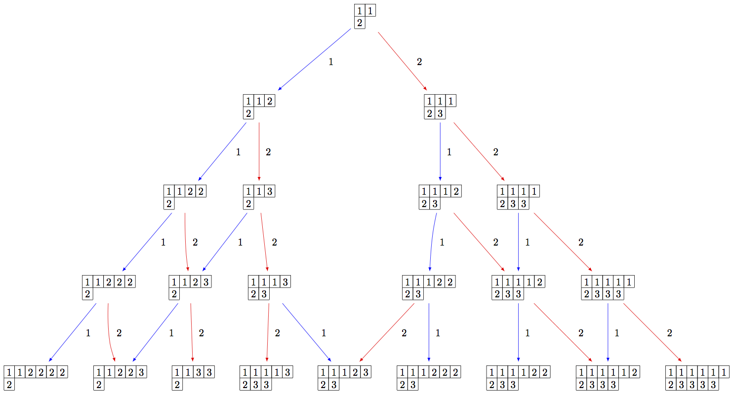
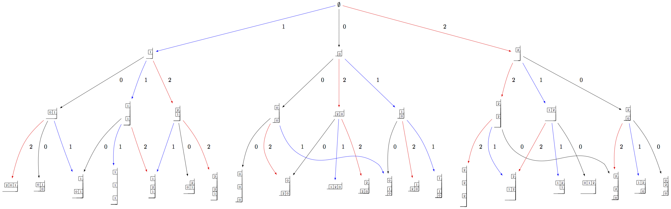
由于晶体是无限的，我们必须指定要查看的子晶体：

sage: B = crystals.infinity.Tableaux(['A',2])
sage: S = B.subcrystal(max_depth=4)
sage: G = B.digraph(subset=S)
sage: view(G, tightpage=True) # optional - dot2tex graphviz, not tested (opens external window)

Using elementary crystals, we can cut irreducible highest weight crystals from B(infty) as the connected component of C otimes T_lambda otimes B(infty) containing cotimes t_lambda otimes u_infty, where u_infty is the highest weight vector in B(infty). In this example, we cut out B(rho) from B(infty) in type A_2:

sage: B = crystals.infinity.Tableaux(['A',2])
sage: b = B.highest_weight_vector()
sage: T = crystals.elementary.T(['A',2], B.Lambda()[1] + B.Lambda()[2])
sage: t = T[0]
sage: C = crystals.elementary.Component(['A',2])
sage: c = C[0]
sage: TP = crystals.TensorProduct(C,T,B)
sage: t0 = TP(c,t,b)
sage: STP = TP.subcrystal(generators=[t0])
sage: GTP = TP.digraph(subset=STP)
sage: view(GTP, tightpage=True) # optional - dot2tex graphviz, not tested (opens external window)

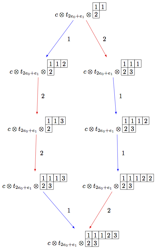
请注意，上面的代码可以使用R-Crystal：：

sage: B = crystals.infinity.Tableaux(['A',2])
sage: b = B.highest_weight_vector()
sage: R = crystals.elementary.R(['A',2], B.Lambda()[1] + B.Lambda()[2])
sage: r = R[0]
sage: TP2 = crystals.TensorProduct(R,B)
sage: t2 = TP2(r,b)
sage: STP2 = TP2.subcrystal(generators=[t2])
sage: GTP2 = TP2.digraph(subset=STP2)
sage: view(GTP2, tightpage=True) # optional - dot2tex graphviz, not tested (opens external window)

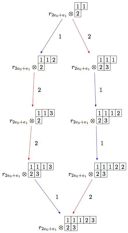
另一方面，我们可以嵌入不可还原的最高重量晶体 B(rho) vt.进入，进入 B(infty) **

sage: Brho = crystals.Tableaux(['A',2],shape=[2,1])
sage: brho = Brho.highest_weight_vector()
sage: B = crystals.infinity.Tableaux(['A',2])
sage: binf = B.highest_weight_vector()
sage: wt = brho.weight()
sage: T = crystals.elementary.T(['A',2],wt)
sage: TlambdaBinf = crystals.TensorProduct(T,B)
sage: hw = TlambdaBinf(T[0],binf)
sage: Psi = Brho.crystal_morphism({brho : hw})
sage: BG = B.digraph(subset=[Psi(x) for x in Brho])
sage: view(BG, tightpage=True) # optional - dot2tex graphviz, not tested (opens external window)

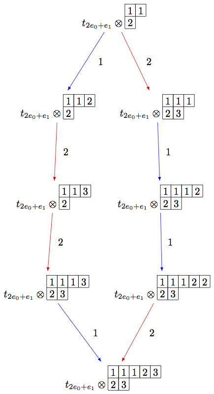
Note that in the last example, we had to inject B(rho) into the tensor product T_lambda otimes B(infty), since otherwise, the map Psi would not be a crystal morphism (as b.weight() != brho.weight()).

广义杨氏墙

J.A.Kim和D.-U Shin提出了广义杨墙作为一种 B(infty) 而且每个人 B(lambda) 仅在仿射型中 A_n^{(1)} 。看见 [KimShin2010] 有关构造广义Young墙的更多信息。

由于此模型仅对一种Cartan类型有效，因此初始化晶体的输入只是基础类型的等级：：

sage: Y = crystals.infinity.GeneralizedYoungWalls(2)
sage: y = Y.highest_weight_vector()
sage: y.f_string([0,1,2,2,2,1,0,0,1,2]).pp()
         2|
          |
          |
       1|2|
       0|1|
 2|0|1|2|0|

在 weight 方法，我们可以选择是在扩展权重晶格(默认情况下)还是在根晶格中查看权重：

sage: Y = crystals.infinity.GeneralizedYoungWalls(2)
sage: y = Y.highest_weight_vector()
sage: y.f_string([0,1,2,2,2,1,0,0,1,2]).weight()
Lambda[0] + Lambda[1] - 2*Lambda[2] - 3*delta
sage: y.f_string([0,1,2,2,2,1,0,0,1,2]).weight(root_lattice=True)
-3*alpha[0] - 3*alpha[1] - 4*alpha[2]

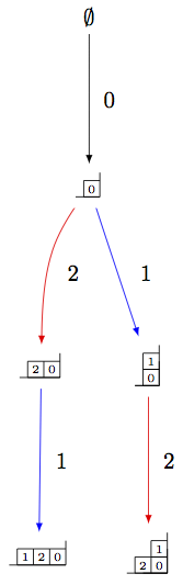
与前面一样，当尝试查看晶图时，我们需要指示特定的亚晶：：

sage: Y = crystals.infinity.GeneralizedYoungWalls(2)
sage: SY = Y.subcrystal(max_depth=3)
sage: GY = Y.digraph(subset=SY)
sage: view(GY, tightpage=True) # optional - dot2tex graphviz, not tested (opens external window)

人们还可以使用广义的Young Wallels制造不可减少的最高重量的晶体：

sage: La = RootSystem(['A',2,1]).weight_lattice(extended=True).fundamental_weights()
sage: YLa = crystals.GeneralizedYoungWalls(2,La[0])
sage: SYLa = YLa.subcrystal(max_depth=3)
sage: GYLa = YLa.digraph(subset=SYLa)
sage: view(GYLa, tightpage=True) # optional - dot2tex graphviz, not tested (opens external window)

然而，在最高权重的晶体中，权重始终是扩展仿射权重晶格的元素：

sage: La = RootSystem(['A',2,1]).weight_lattice(extended=True).fundamental_weights()
sage: YLa = crystals.GeneralizedYoungWalls(2,La[0])
sage: YLa.highest_weight_vector().f_string([0,1,2,0]).weight()
-Lambda[0] + Lambda[1] + Lambda[2] - 2*delta

修正Nakajima单项式

Let Y_{i,k}, for i in I and k in ZZ, be a commuting set of variables, and let boldsymbol{1} be a new variable which commutes with each Y_{i,k}. (Here, I represents the index set of a Cartan datum.) One may endow the structure of a crystal on the set widehat{mathcal{M}} of monomials of the form

\[M = \prod_{(i,k) \in I\times \ZZ_{\ge0}} Y_{i,k}^{y_i(k)}\boldsymbol{1}.\]

Elements of widehat{mathcal{M}} are called modified Nakajima monomials. We will omit the boldsymbol{1} from the end of a monomial if there exists at least one y_i(k) neq 0. The crystal structure on this set is defined by

\[\begin{split}\begin{aligned} \mathrm{wt}(M) &= \sum_{i\in I} \Bigl( \sum_{k\ge 0} y_i(k) \Bigr) \Lambda_i, \\ \varphi_i(M) &= \max\Bigl\{ \sum_{0\le j \le k} y_i(j) : k\ge 0 \Bigr\}, \\ \varepsilon_i(M) &= \varphi_i(M) - \langle h_i, \mathrm{wt}(M) \rangle, \\ k_f = k_f(M) &= \min\Bigl\{ k\ge 0 : \varphi_i(M) = \sum_{0\le j\le k} y_i(j) \Bigr\}, \\ k_e = k_e(M) &= \max\Bigl\{ k\ge 0 : \varphi_i(M) = \sum_{0\le j\le k} y_i(j) \Bigr\}, \end{aligned}\end{split}\]

where {h_i : i in I} and {Lambda_i : i in I } are the simple coroots and fundamental weights, respectively. With a chosen set of integers C = (c_{ij})_{ineq j} such that c_{ij}+c_{ji} =1, one defines

\[A_{i，k}=Y_{i，k}Y_{i，k+1}\prod_{j\neq i}Y_{j，k+c_{ji}^{a_{ji}}，\]

哪里 (a_{ij}) 是一个Cartan矩阵。然后

\[\begin{split}\begin{aligned} e_iM &= \begin{cases} 0 & \text{if } \varepsilon_i(M) = 0, \\ A_{i,k_e}M & \text{if } \varepsilon_i(M) > 0, \end{cases} \\ f_iM &= A_{i,k_f}^{-1} M. \end{aligned}\end{split}\]

备注

单项晶体取决于正整数的选择 C = (c_{ij})_{ineq j} 满足条件 c_{ij}+c_{ji}=1 。这个选择在Sage中做出了这样的选择 c_{ij} = 1 如果 i < j 和 c_{ij} = 0 如果 i>j ，但如果在晶体初始化时有意说明，也可以使用其他选项：

sage: c = Matrix([[0,0,1],[1,0,0],[0,1,0]])
sage: La = RootSystem(['C',3]).weight_lattice().fundamental_weights()
sage: M = crystals.NakajimaMonomials(2*La[1], c=c)
sage: M.c()
[0 0 1]
[1 0 0]
[0 1 0]

It is shown in [KKS2007] that the connected component of widehat{mathcal{M}} containing the element boldsymbol{1}, which we denote by mathcal{M}(infty), is crystal isomorphic to the crystal B(infty):

sage: Minf = crystals.infinity.NakajimaMonomials(['C',3,1])
sage: minf = Minf.highest_weight_vector()
sage: m = minf.f_string([0,1,2,3,2,1,0]); m
Y(0,0)^-1 Y(0,4)^-1 Y(1,0) Y(1,3)
sage: m.weight()
-2*Lambda[0] + 2*Lambda[1] - 2*delta
sage: m.weight_in_root_lattice()
-2*alpha[0] - 2*alpha[1] - 2*alpha[2] - alpha[3]

我们也可以做模特 B(infty) 使用变量 A_{i,k} 相反：：

sage: Minf = crystals.infinity.NakajimaMonomials(['C',3,1])
sage: minf = Minf.highest_weight_vector()
sage: Minf.set_variables('A')
sage: m = minf.f_string([0,1,2,3,2,1,0]); m
A(0,0)^-1 A(0,3)^-1 A(1,0)^-1 A(1,2)^-1 A(2,0)^-1 A(2,1)^-1 A(3,0)^-1
sage: m.weight()
-2*Lambda[0] + 2*Lambda[1] - 2*delta
sage: m.weight_in_root_lattice()
-2*alpha[0] - 2*alpha[1] - 2*alpha[2] - alpha[3]
sage: Minf.set_variables('Y')

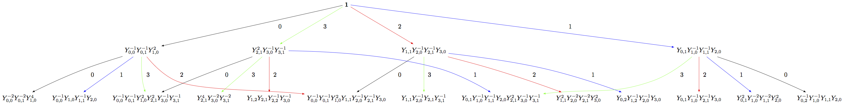
构建这些单项晶体的晶图输出与上面的构造相同：

sage: Minf = crystals.infinity.NakajimaMonomials(['C',3,1])
sage: Sinf = Minf.subcrystal(max_depth=2)
sage: Ginf = Minf.digraph(subset=Sinf)
sage: view(Ginf, tightpage=True) # optional - dot2tex graphviz, not tested (opens external window)

请注意，该模型也适用于任何可对称化的Cartan矩阵：

sage: A = CartanMatrix([[2,-4],[-5,2]])
sage: Linf = crystals.infinity.NakajimaMonomials(A); Linf
Infinity Crystal of modified Nakajima monomials of type [ 2 -4]
[-5  2]
sage: Linf.highest_weight_vector().f_string([0,1,1,1,0,0,1,1,0])
Y(0,0)^-1 Y(0,1)^9 Y(0,2)^5 Y(0,3)^-1 Y(1,0)^2 Y(1,1)^5 Y(1,2)^3

受操纵的配置

操纵配置是分区序列，底层动态关系图中的每个节点对应一个分区，因此每个分区的每个部分都有一个标签(或操纵)。在这些物体上定义了晶体结构 [Schilling2006], 后来扩展到作为模型工作 B(infty) 。看见 [SalisburyScrimshaw2015] 有关更多信息，请访问：

sage: RiggedConfigurations.options(display="horizontal")
sage: RC = crystals.infinity.RiggedConfigurations(['C',3,1])
sage: nu = RC.highest_weight_vector().f_string([0,1,2,3,2,1,0]); nu
-2[ ]-1   2[ ]1   0[ ]0   0[ ]0
-2[ ]-1   2[ ]1   0[ ]0
sage: nu.weight()
-2*Lambda[0] + 2*Lambda[1] - 2*delta
sage: RiggedConfigurations.options._reset()

我们可以使用Nakajima单项式检查此晶体是否与上面的晶体同构：：

sage: Minf = crystals.infinity.NakajimaMonomials(['C',3,1])
sage: Sinf = Minf.subcrystal(max_depth=2)
sage: Ginf = Minf.digraph(subset=Sinf)
sage: RC = crystals.infinity.RiggedConfigurations(['C',3,1])
sage: RCS = RC.subcrystal(max_depth=2)
sage: RCG = RC.digraph(subset=RCS)
sage: RCG.is_isomorphic(Ginf, edge_labels=True)
True

该模型在Sage中适用于所有有限和仿射类型，以及任何简单花边Cartan矩阵。