仿射有限晶体

在这份文件中，我们简要地解释了基里洛夫-雷希蒂欣晶体的结构和实现 [FourierEtAl2009].

Kirillov--Reshetikhin (KR) crystals are finite-dimensional affine crystals corresponding to Kirillov--Reshektikhin modules. They were first conjectured to exist in [HatayamaEtAl2001]. The proof of their existence for nonexceptional types was given in [OkadoSchilling2008] and their combinatorial models were constructed in [FourierEtAl2009]. Kirillov-Reshetikhin crystals B^{r,s} are indexed first by their type (like A_n^{(1)}, B_n^{(1)}, ...) with underlying index set I = {0,1,ldots, n} and two integers r and s. The integers s only needs to satisfy s >0, whereas r is a node of the finite Dynkin diagram r in I setminus {0}.

它们的构建依赖于几个案例，我们将分别讨论这些案例。在所有情况下，当移除零箭头时，晶体分解为经典晶体的(直和)，这给出了指数集的晶体结构 I_0 = { 1,2,ldots, n} 。然后，通过利用动态金图的对称性或通过嵌入晶体来添加零箭头。

类型 A_n^{(1)}

仿射型的动态图 A 具有旋转对称映射 sigma: i mapsto i+1 在这里我们查看模数的指数 n+1 **

sage: C = CartanType(['A',3,1])
sage: C.dynkin_diagram()
0
O-------+
|       |
|       |
O---O---O
1   2   3
A3~

的经典分解 B^{r,s} 是 A_n 最高重量晶体 B(somega_r) 或者相当于由矩形隔板标记的画面的晶体 (s^r) ：

\[B^{r,s} \cong B(s\omega_r) \quad \text{as a } \{1,2,\ldots,n\}\text{-crystal}\]

在Sage中，我们可以通过：：

sage: K = crystals.KirillovReshetikhin(['A',3,1],1,1)
sage: K.classical_decomposition()
The crystal of tableaux of type ['A', 3] and shape(s) [[1]]
sage: K.list()
[[[1]], [[2]], [[3]], [[4]]]

sage: K = crystals.KirillovReshetikhin(['A',3,1],2,1)
sage: K.classical_decomposition()
The crystal of tableaux of type ['A', 3] and shape(s) [[1, 1]]

人们可以使用这些方法在经典晶体和仿射晶体之间进行转换 lift 和 retract **

sage: K = crystals.KirillovReshetikhin(['A',3,1],2,1)
sage: b = K(rows=[[1],[3]]); type(b)
<class 'sage.combinat.crystals.kirillov_reshetikhin.KR_type_A_with_category.element_class'>
sage: b.lift()
[[1], [3]]
sage: type(b.lift())
<class 'sage.combinat.crystals.tensor_product.CrystalOfTableaux_with_category.element_class'>

sage: b = crystals.Tableaux(['A',3], shape = [1,1])(rows=[[1],[3]])
sage: K.retract(b)
[[1], [3]]
sage: type(K.retract(b))
<class 'sage.combinat.crystals.kirillov_reshetikhin.KR_type_A_with_category.element_class'>

这个 0 -箭头是使用类似于 sigma ，被称为促销操作员 mathrm{pr} ，在晶体水平上，通过：

\[ \begin{align}\begin{aligned}f_0 = \mathrm{pr}^{-1} \circ f_1 \circ \mathrm{pr}\\e_0 = \mathrm{pr}^{-1} \circ e_1 \circ \mathrm{pr}\end{aligned}\end{align} \]

在Sage中，这可以通过以下方式实现：

sage: K = crystals.KirillovReshetikhin(['A',3,1],2,1)
sage: b = K.module_generator(); b
[[1], [2]]
sage: b.f(0)
sage: b.e(0)
[[2], [4]]

sage: K.promotion()(b.lift())
[[2], [3]]
sage: K.promotion()(b.lift()).e(1)
[[1], [3]]
sage: K.promotion_inverse()(K.promotion()(b.lift()).e(1))
[[2], [4]]

KR晶体是水平的 0 晶体，这意味着这些晶体中所有元素的重量为零：：

sage: K = crystals.KirillovReshetikhin(['A',3,1],2,1)
sage: b = K.module_generator(); b.weight()
-Lambda[0] + Lambda[2]
sage: b.weight().level()
0

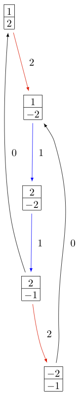
KR晶体 B^{1,1} 类型的 A_2^{(1)} 如下所示：

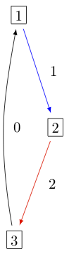
在Sage中，可以通过：：

sage: K = crystals.KirillovReshetikhin(['A',2,1],1,1)
sage: G = K.digraph()
sage: view(G, tightpage=True) # optional - dot2tex graphviz, not tested (opens external window)

类型 D_n^{(1)} ， B_n^{(1)} ， A_{2n-1}^{(2)}

类型的动态图 D_n^{(1)} ， B_n^{(1)} ， A_{2n-1}^{(2)} 在互换节点下是不变的 0 和 1 **

sage: n = 5
sage: C = CartanType(['D',n,1]); C.dynkin_diagram()
  0 O   O 5
    |   |
    |   |
O---O---O---O
1   2   3   4
D5~
sage: C = CartanType(['B',n,1]); C.dynkin_diagram()
    O 0
    |
    |
O---O---O---O=>=O
1   2   3   4   5
B5~
sage: C = CartanType(['A',2*n-1,2]); C.dynkin_diagram()
    O 0
    |
    |
O---O---O---O=<=O
1   2   3   4   5
B5~*

去掉结点时得到的下标经典代数 0 是类型 mathfrak{g}_0 = D_n, B_n, C_n ，分别为。将经典分解成一个 mathfrak{g}_0 Crystal是一个直接总和：

\[B^{r,s} \cong \bigoplus_\lambda B(\lambda) \quad \text{as a } \{1,2,\ldots,n\}\text{-crystal}\]

where lambda is obtained from somega_r (or equivalently a rectangular partition of shape (s^r)) by removing vertical dominoes. This in fact only holds in the ranges 1le rle n-2 for type D_n^{(1)}, and 1 le r le n for types B_n^{(1)} and A_{2n-1}^{(2)}:

sage: K = crystals.KirillovReshetikhin(['D',6,1],4,2)
sage: K.classical_decomposition()
The crystal of tableaux of type ['D', 6] and shape(s)
 [[], [1, 1], [1, 1, 1, 1], [2, 2], [2, 2, 1, 1], [2, 2, 2, 2]]

对于类型 B_n^{(1)} 和 r=n ，人们需要意识到 omega_n 是自旋权重，因此在划分语言中对应于一列高度 n 和宽度 1/2 **

sage: K = crystals.KirillovReshetikhin(['B',3,1],3,1)
sage: K.classical_decomposition()
The crystal of tableaux of type ['B', 3] and shape(s) [[1/2, 1/2, 1/2]]

至于类型 A_n^{(1)} ，动态自同构导出了一个升级型算子 sigma 在晶体的层面上。然而，在这种情况下，可能会发生经典组件之间的自同构改变：

sage: K = crystals.KirillovReshetikhin(['D',4,1],2,1)
sage: b = K.module_generator(); b
[[1], [2]]
sage: K.automorphism(b)
[[2], [-1]]
sage: b = K(rows=[[2],[-2]])
sage: K.automorphism(b)
[]

此运算符 sigma 用于定义仿射晶体运算符：

\[ \begin{align}\begin{aligned}f_0 = \sigma \circ f_1 \circ \sigma\\e_0 = \sigma \circ e_1 \circ \sigma\end{aligned}\end{align} \]

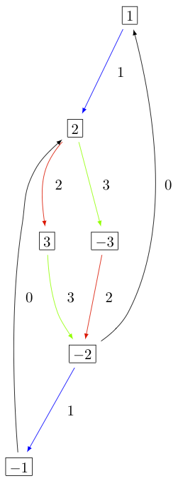
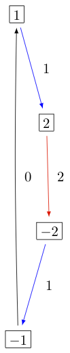
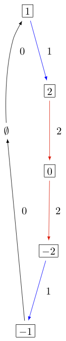
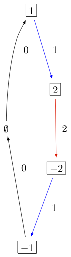
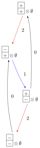
KR晶体 B^{1,1} 类型的 D_3^{(1)} ， B_2^{(1)} ，以及 A_5^{(2)} 它们分别是：

类型 C_n^{(1)}

活字的动态图解 C_n^{(1)} 具有对称性 sigma(i) = n-i **

sage: C = CartanType(['C',4,1]); C.dynkin_diagram()
O=>=O---O---O=<=O
0   1   2   3   4
C4~

去掉0结点时的经典子代数是 C_n 。

然而，在这种情况下，水晶 B^{r,s} 不是使用 sigma ，而是使用虚拟晶体结构。 B^{r,s} 类型的 C_n^{(1)} 是在内部实现的 hat{V}^{r,s} 类型的 A_{2n+1}^{(2)} 使用：

\[ \begin{align}\begin{aligned}e_0 = \hat{e}_0 \hat{e}_1 \quad \text{and} \quad e_i = \hat{e}_{i+1} \quad \text{for} \quad 1\le i\le n\\f_0 = \hat{f}_0 \hat{f}_1 \quad \text{and} \quad f_i = \hat{f}_{i+1} \quad \text{for} \quad 1\le i\le n\end{aligned}\end{align} \]

哪里 hat{e}_i 和 hat{f}_i 是环境晶体中的晶体运算符 hat{V}^{r,s} **

sage: K = crystals.KirillovReshetikhin(['C',3,1],1,2); K.ambient_crystal()
Kirillov-Reshetikhin crystal of type ['B', 4, 1]^* with (r,s)=(1,2)

的经典分解 1 le r < n 由以下人员提供：

\[B^{r,s} \cong \bigoplus_\lambda B(\lambda) \quad \text{as a } \{1,2,\ldots,n\}\text{-crystal}\]

哪里 lambda 从以下来源获得 somega_r (或者相当于形状的矩形隔板 (s^r) )通过移除水平多米诺骨牌：

sage: K = crystals.KirillovReshetikhin(['C',3,1],2,4)
sage: K.classical_decomposition()
The crystal of tableaux of type ['C', 3] and shape(s) [[], [2], [4], [2, 2], [4, 2], [4, 4]]

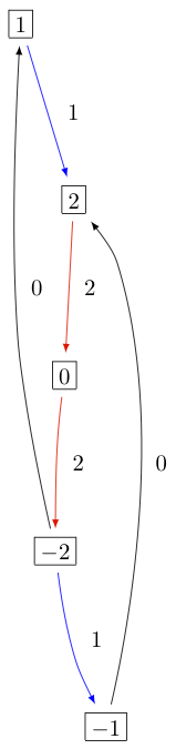
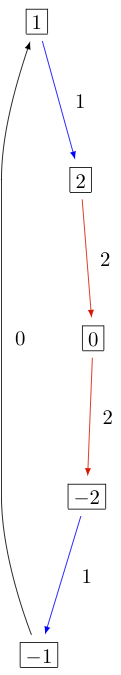
KR晶体 B^{1,1} 类型的 C_2^{(1)} 如下所示：

类型 D_{n+1}^{(2)} ， A_{2n}^{(2)}

类型的动态图 D_{n+1}^{(2)} 和 A_{2n}^{(2)} 外观如下：

sage: C = CartanType(['D',5,2]); C.dynkin_diagram()
O=<=O---O---O=>=O
0   1   2   3   4
C4~*

sage: C = CartanType(['A',8,2]); C.dynkin_diagram()
O=<=O---O---O=<=O
0   1   2   3   4
BC4~

经典的子图是这样的 B_n 对于类型 D_{n+1}^{(2)} 和类型 C_n 对于类型 A_{2n}^{(2)} 。这些KR晶体的经典分解 1le r < n 对于类型 D_{n+1}^{(2)} 和 1 le r le n 对于类型 A_{2n}^{(2)} 由以下人员提供：

\[B^{r,s} \cong \bigoplus_\lambda B(\lambda) \quad \text{as a } \{1,2,\ldots,n\}\text{-crystal}\]

哪里 lambda 从以下来源获得 somega_r (或者相当于形状的矩形隔板 (s^r) )通过删除单个框：：

sage: K = crystals.KirillovReshetikhin(['D',5,2],2,2)
sage: K.classical_decomposition()
The crystal of tableaux of type ['B', 4] and shape(s) [[], [1], [2], [1, 1], [2, 1], [2, 2]]

sage: K = crystals.KirillovReshetikhin(['A',8,2],2,2)
sage: K.classical_decomposition()
The crystal of tableaux of type ['C', 4] and shape(s) [[], [1], [2], [1, 1], [2, 1], [2, 2]]

KR晶体使用到类型为KR的KR晶体的内射映射来构造 C_n^{(1)}

\[S : B^{r,s} \to B^{r,2s}_{C_n^{(1)}} \quad \text{such that } S(e_ib) = e_i^{m_i}S(b) \text{ and } S(f_ib) = f_i^{m_i}S(b)\]

哪里

\[(m_0,\ldots,m_n) = (1,2,\ldots,2,1) \text{ for type } D_{n+1}^{(2)} \quad \text{and} \quad (1,2,\ldots,2,2) \text{ for type } A_{2n}^{(2)}.\]

sage: K = crystals.KirillovReshetikhin(['D',5,2],1,2); K.ambient_crystal()
Kirillov-Reshetikhin crystal of type ['C', 4, 1] with (r,s)=(1,4)
sage: K = crystals.KirillovReshetikhin(['A',8,2],1,2); K.ambient_crystal()
Kirillov-Reshetikhin crystal of type ['C', 4, 1] with (r,s)=(1,4)

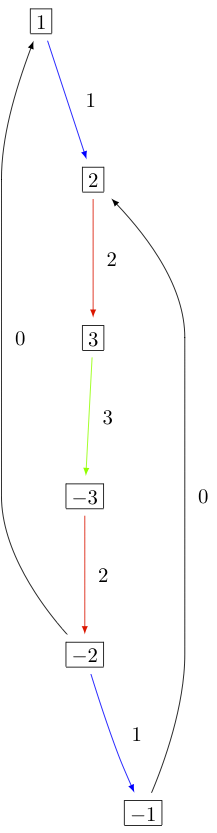
KR晶体 B^{1,1} 类型的 D_3^{(2)} 和 A_4^{(2)} 外观如下：

正如您可以从类型的动态关系图中看到的 A_{2n}^{(2)} ，映射节点 imapsto n-i 生成相同的图表，但节点已重新标记。在这种情况下，经典子图的类型为 B_n 而不是 C_n 。人们还可以构建KR晶体 B^{r,s} 类型的 A_{2n}^{(2)} 基于这一经典分解。在这种情况下，经典分解是从 s omega_r 通过移除水平多米诺骨牌：

sage: C = CartanType(['A',6,2]).dual()
sage: Kdual = crystals.KirillovReshetikhin(C,2,2)
sage: Kdual.classical_decomposition()
The crystal of tableaux of type ['B', 3] and shape(s) [[], [2], [2, 2]]

从图中可以看出，此实现与基于 C_n 分解到重新标记箭头：：

sage: C = CartanType(['A',4,2])
sage: K = crystals.KirillovReshetikhin(C,1,1)
sage: Kdual = crystals.KirillovReshetikhin(C.dual(),1,1)
sage: G = K.digraph()
sage: Gdual = Kdual.digraph()
sage: f = { 1:1, 0:2, 2:0 }
sage: for u,v,label in Gdual.edges(sort=False):
....:     Gdual.set_edge_label(u,v,f[label])
sage: G.is_isomorphic(Gdual, edge_labels = True)
True

异常节点

KR晶体 B^{n,s} 对于类型 C_n^{(1)} 和 D_{n+1}^{(2)} 被排除在上述讨论之外。它们与异常节点相关联 r=n 在这种情况下，经典分解是不可约的：

\[B^{n，S}\从B(S\omega_n)。\]

在Sage：：

sage: K = crystals.KirillovReshetikhin(['C',2,1],2,1)
sage: K.classical_decomposition()
The crystal of tableaux of type ['C', 2] and shape(s) [[1, 1]]

sage: K = crystals.KirillovReshetikhin(['D',3,2],2,1)
sage: K.classical_decomposition()
The crystal of tableaux of type ['B', 2] and shape(s) [[1/2, 1/2]]

KR晶体 B^{n,s} 和 B^{n-1,s} 类型的 D_n^{(1)} 也很特别。它们分解为：

\[B^{n,s} \cong B(s\omega_n) \quad \text{ and } \quad B^{n-1,s} \cong B(s\omega_{n-1}).\]

sage: K = crystals.KirillovReshetikhin(['D',4,1],4,1)
sage: K.classical_decomposition()
The crystal of tableaux of type ['D', 4] and shape(s) [[1/2, 1/2, 1/2, 1/2]]
sage: K = crystals.KirillovReshetikhin(['D',4,1],3,1)
sage: K.classical_decomposition()
The crystal of tableaux of type ['D', 4] and shape(s) [[1/2, 1/2, 1/2, -1/2]]

类型 E_6^{(1)}

In [JonesEtAl2010] the KR crystals B^{r,s} for r=1,2,6 in type E_6^{(1)} were constructed exploiting again a Dynkin diagram automorphism, namely the automorphism sigma of order 3 which maps 0mapsto 1 mapsto 6 mapsto 0:

sage: C = CartanType(['E',6,1]); C.dynkin_diagram()
        O 0
        |
        |
        O 2
        |
        |
O---O---O---O---O
1   3   4   5   6
E6~

水晶 B^{1,s} 和 B^{6,s} 像经典晶体一样不可还原：：

sage: K = crystals.KirillovReshetikhin(['E',6,1],1,1)
sage: K.classical_decomposition()
Direct sum of the crystals Family (Finite dimensional highest weight crystal of type ['E', 6] and highest weight Lambda[1],)
sage: K = crystals.KirillovReshetikhin(['E',6,1],6,1)
sage: K.classical_decomposition()
Direct sum of the crystals Family (Finite dimensional highest weight crystal of type ['E', 6] and highest weight Lambda[6],)

而对于伴随节点 r=2 我们有腐烂的东西

\[B^{2，S}\cong\Bigoplus_{k=0}^S B(k\omega_2)\]

sage: K = crystals.KirillovReshetikhin(['E',6,1],2,1)
sage: K.classical_decomposition()
Direct sum of the crystals Family (Finite dimensional highest weight crystal of type ['E', 6] and highest weight 0,
Finite dimensional highest weight crystal of type ['E', 6] and highest weight Lambda[2])

对应的晶体上的提升运算符 sigma 可以显式计算：

sage: K = crystals.KirillovReshetikhin(['E',6,1],1,1)
sage: promotion = K.promotion()
sage: u = K.module_generator(); u
[(1,)]
sage: promotion(u.lift())
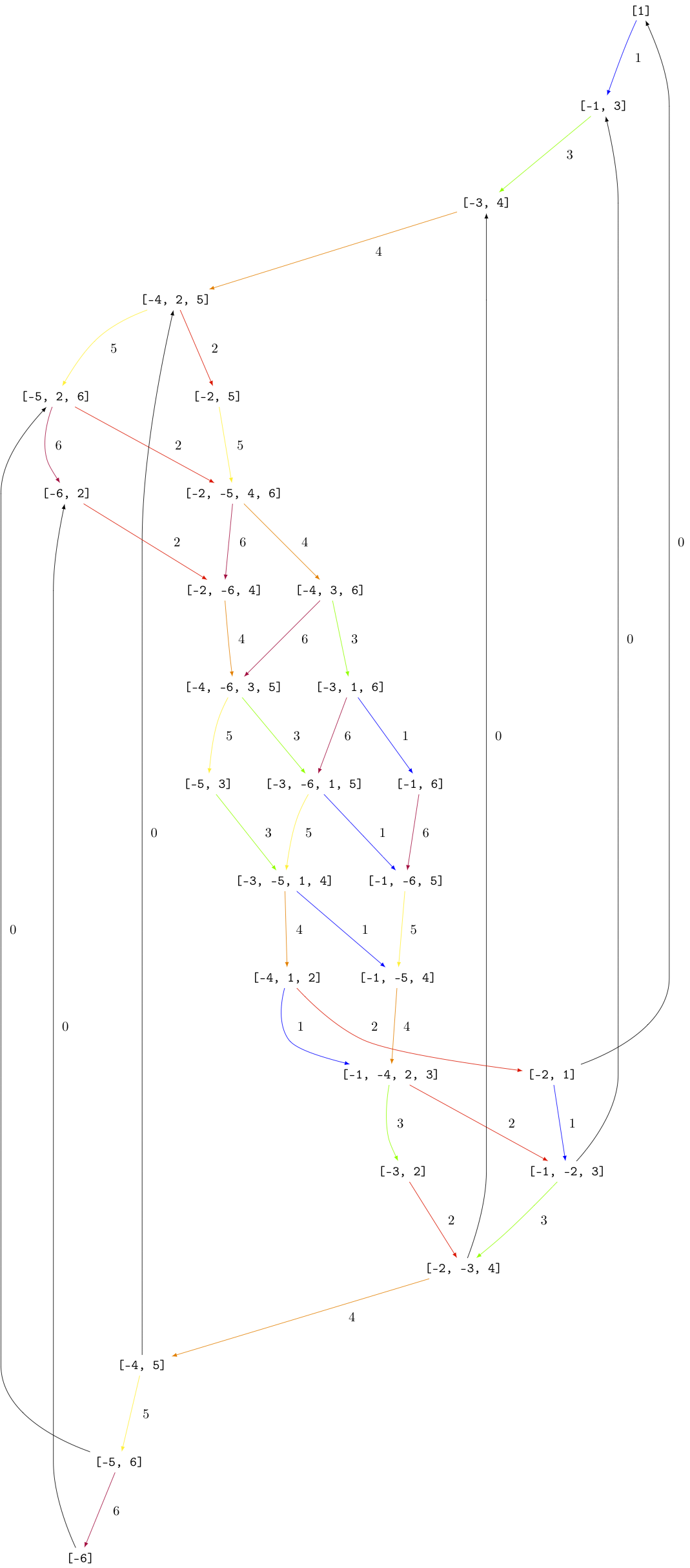
[(-1, 6)]

The crystal B^{1,1} is already of dimension 27. The elements b of this crystal are labelled by tuples which specify their nonzero phi_i(b) and epsilon_i(b). For example, [-6,2] indicates that phi_2([-6,2]) = epsilon_6([-6,2]) = 1 and all others are equal to zero:

sage: K = crystals.KirillovReshetikhin(['E',6,1],1,1)
sage: K.cardinality()
27

单柱KR晶体

单柱KR晶体是 B^{r,1} 对于任何 r in I_0 。

在……里面 [LNSSS14I] 和 [LNSSS14II], 结果表明，通过将LS路径的0级晶体投影到经典的重量晶格上，可以构造出单柱KR晶体。我们首先验证我们确实得到了一个同构的晶体 B^{1,1} 输入文字 E_6^{(1)} **

sage: K = crystals.KirillovReshetikhin(['E',6,1], 1,1)
sage: K2 = crystals.kirillov_reshetikhin.LSPaths(['E',6,1], 1,1)
sage: K.digraph().is_isomorphic(K2.digraph(), edge_labels=True)
True

下面是一个例子 E_8^{(1)} 我们计算了它的经典分解：

sage: K = crystals.kirillov_reshetikhin.LSPaths(['E',8,1], 8,1)
sage: K.cardinality()
249
sage: L = [x for x in K if x.is_highest_weight([1,2,3,4,5,6,7,8])]
sage: [x.weight() for x in L]
[-2*Lambda[0] + Lambda[8], 0]

应用

有限维仿射晶体的一个重要概念是完美性。关键的性质是一种晶体 B 是完美的水平 ell 如果在级别之间存在双射 ell 中的主要权重和元素

\[B_{\mathrm{min}} = \{ b \in B \mid \mathrm{lev}(\varphi(b)) = \ell \}\;.\]

有关完美晶体的准确定义，请参阅 [HongKang2002] 。在……里面 [FourierEtAl2010] 事实证明，对于非异常类型 B^{r,s} 是完美的，只要 s/c_r 是一个整数。这里 c_r=1 除 c_r=2 为 1 le r < n 输入文字 C_n^{(1)} 和 r=n 输入文字 B_n^{(1)} 。

在这里，我们使用Sage for进行验证 B^{1,1} 类型的 C_3^{(1)} **

sage: K = crystals.KirillovReshetikhin(['C',3,1],1,1)
sage: Lambda = K.weight_lattice_realization().fundamental_weights(); Lambda
Finite family {0: Lambda[0], 1: Lambda[1], 2: Lambda[2], 3: Lambda[3]}
sage: [w.level() for w in Lambda]
[1, 1, 1, 1]
sage: Bmin = [b for b in K if b.Phi().level() == 1 ]; Bmin
[[[1]], [[2]], [[3]], [[-3]], [[-2]], [[-1]]]
sage: [b.Phi() for b in Bmin]
[Lambda[1], Lambda[2], Lambda[3], Lambda[2], Lambda[1], Lambda[0]]

如你所见，两者 b=1 和 b=-2 满足 varphi(b)=Lambda_1 。因此，中的最小元素之间不存在双向映射 B_{mathrm{min}} 和1级权重。因此， B^{1,1} 类型的 C_3^{(1)} 并不完美。然而， B^{1,2} 类型的 C_n^{(1)} 是一块完美的水晶：：

sage: K = crystals.KirillovReshetikhin(['C',3,1],1,2)
sage: Lambda = K.weight_lattice_realization().fundamental_weights()
sage: Bmin = [b for b in K if b.Phi().level() == 1 ]
sage: [b.Phi() for b in Bmin]
[Lambda[0], Lambda[3], Lambda[2], Lambda[1]]

利用京都路径模型，完全晶体可以用来构造无限维的最高重量晶体和去蓝晶体 [KKMMNN1992]. 我们在中构造了示例10.6.5 [HongKang2002]:

sage: K = crystals.KirillovReshetikhin(['A',1,1], 1,1)
sage: La = RootSystem(['A',1,1]).weight_lattice().fundamental_weights()
sage: B = crystals.KyotoPathModel(K, La[0])
sage: B.highest_weight_vector()
[[[2]]]

sage: K = crystals.KirillovReshetikhin(['A',2,1], 1,1)
sage: La = RootSystem(['A',2,1]).weight_lattice().fundamental_weights()
sage: B = crystals.KyotoPathModel(K, La[0])
sage: B.highest_weight_vector()
[[[3]]]

sage: K = crystals.KirillovReshetikhin(['C',2,1], 2,1)
sage: La = RootSystem(['C',2,1]).weight_lattice().fundamental_weights()
sage: B = crystals.KyotoPathModel(K, La[1])
sage: B.highest_weight_vector()
[[[2], [-2]]]

能量函数与一维构型和

对于Kirillov-Reshehtikhin晶体的张量积，也存在重要的能量函数概念。它可以定义为某些局部能量函数和 R -矩阵。在中的定理7.5中 [SchillingTingley2011] 结果表明，对于相同能级的完美晶体，能量 D(b) 与仿射分级相同(直到规格化)。仿射分级被定义为最小应用次数 e_0 至 b 才能到达基态路径。在计算上，该算法比涉及 R -矩阵，并已在Sage：：

sage: K = crystals.KirillovReshetikhin(['A',2,1],1,1)
sage: T = crystals.TensorProduct(K,K,K)
sage: hw = [b for b in T if all(b.epsilon(i)==0 for i in [1,2])]
sage: for b in hw:
....:     print("{} {}".format(b, b.energy_function()))
[[[1]], [[1]], [[1]]] 0
[[[1]], [[2]], [[1]]] 2
[[[2]], [[1]], [[1]]] 1
[[[3]], [[2]], [[1]]] 3

即使对于不完美的晶体，也可以计算仿射分级：

sage: K = crystals.KirillovReshetikhin(['C',4,1],1,2)
sage: K1 = crystals.KirillovReshetikhin(['C',4,1],1,1)
sage: T = crystals.TensorProduct(K,K1)
sage: hw = [b for b in T if all(b.epsilon(i)==0 for i in [1,2,3,4])]
sage: for b in hw:
....:     print("{} {}".format(b, b.affine_grading()))
[[], [[1]]] 1
[[[1, 1]], [[1]]] 2
[[[1, 2]], [[1]]] 1
[[[1, -1]], [[1]]] 0

晶体的一维构型和 B 是所有元素的重量的能量分级和吗？ b in B ：

\[X(B)=\sum_{b\in B}x^{\mathm{Weight}(B)}q^{D(B)}\]

以下是如何在Sage中计算一维配置总和的示例：

sage: K = crystals.KirillovReshetikhin(['A',2,1],1,1)
sage: T = crystals.TensorProduct(K,K)
sage: T.one_dimensional_configuration_sum()
B[-2*Lambda[1] + 2*Lambda[2]] + (q+1)*B[-Lambda[1]]
 + (q+1)*B[Lambda[1] - Lambda[2]] + B[2*Lambda[1]]
 + B[-2*Lambda[2]] + (q+1)*B[Lambda[2]]