遥感教程第一节考试
目录

考试1
这是本教程中两个主要的解释性考试中的第一个,尽管后面的部分将有相当多的问题。与之前的问题不同的是,这里的大部分内容将与这一特殊小节中包含的图像和地图相关,这一小节是从作者1982年的(NMS)中绘制的。 陆地卫星教学手册 . 它们都与一个单一的区域场景有关,包括宾夕法尼亚州中南部的大部分地区,以及特拉华州和马里兰州的一些小部分。大多数图像是由陆地卫星MSS拍摄的(记住,波段4=光谱的绿色部分;波段5=红色部分;6和7=近红外部分)。两个热成像和两个雷达图像,由其他传感器系统,也被使用。一些图像产品是计算机衍生的输出,如空间过滤图像和分类。
我们首先展示了一个由气象卫星上的AVHRR传感器拍摄的整个状态的卫星视图。为了好玩,找到匹兹堡和费城(它们以浅蓝色出现)。
然后,为了将我们正在研究的区域设置为背景,我们将根据国家DEM(数字高程模型)数据制作的高程(红色更高)彩色再现图,从地形的角度来观察该州的大部分东部地区。将随后的场景作为参考,也将其放入上面的AVHRR图像中。
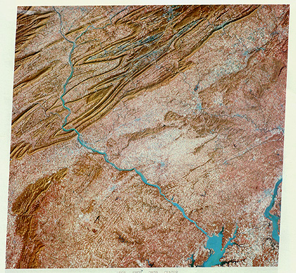
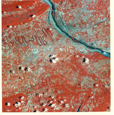
现在,我们从MSS 5图像开始,以接近1:1000000的比例在您的屏幕上复制,这是NASA和其他机构分发的图像的标准尺寸,并在商业上出售。下面是相应的MSS 7图像。下面是同一场景的假彩色合成。1972年10月11日,一场大风暴袭击了美国东北部的大部分地区,最南边是弗吉尼亚州南部,之后一天,所有这些地区都被收购。天晴后,空气特别清新干燥,减少了现场水分的降解作用。
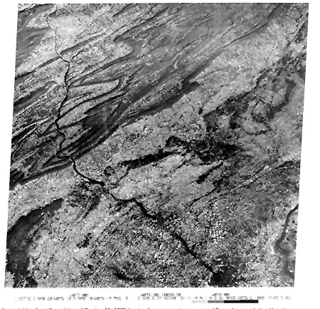

1-1: ` <>`__ Using all three images, but especially the Band 7 image, with the help of an atlas or AAA Road Map, locate the following towns and other features: Harrisburg, York, Gettysburg, Lancaster, Hershey, Lebanon, Reading, Allentown, Easton, Wilmington, DE, the Susquehanna River, the Delaware River; the Juniata River. Also, look hard for the small (15000+) town, Bloomsburg, PA ,which is the current home of the writer (NMS), where this question is being written. `ANSWER <../Sect01/exama.html#1-1>`__
1-2: ` <>`__ What other towns, rivers, or natural features and points of interest in this scene can you list?`ANSWER <../Sect01/exama.html#1-2>`__
`**1-3:** <>`__ **What band(s) seems best for picking out the towns and rivers in each of the images? What is MSS 5 especially good at bringing to your attention. ANSWER **
为了让您感受到图片中山脊部分的典型外观,请浏览这张拍摄于蓝山以北约15公里(10英里)的地面照片,蓝山是从黎巴嫩山谷向北遇到的第一条主要山脊。这片区域拍摄于1999年2月的一天,当时树木光秃秃的,沿着81号州际公路,靠近陆地卫星图像的中心。
现在,看看下面的地质图的黑白印刷图,它覆盖了大部分场景,以及一些周围区域。
`**1-4:** <>`__ **Fit the major rock unit patterns to the Band 5 image. Comment on the fit. ANSWER **
`**1-5:** <>`__ **Comment on what may be unusual about (the color in) the false color composite. ANSWER **
`**1-6:** <>`__ **You may have noted that there is a strip of notation at the bottom of both the individual band images and the false color composite. This is on nearly all renditions of Landsat images regardless of the printed size. We will reproduce this strip, enlarged a bit, just below. Make an educated guess as to what the different groupings of letters/numbers mean. ANSWER **
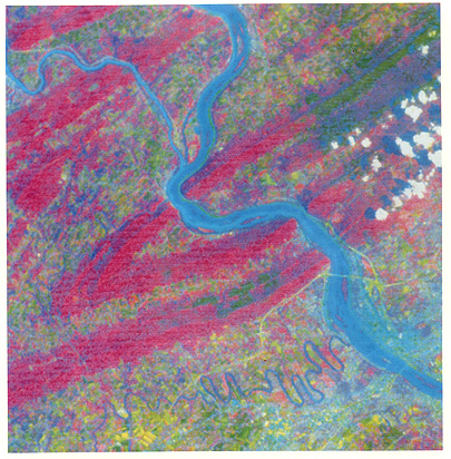
接下来,熟悉1975年10月23日同一区域的假彩色合成图。
`**1-7:** <>`__ **What overall is different and why? Account for the blue in the Susquehanna River. ANSWER **
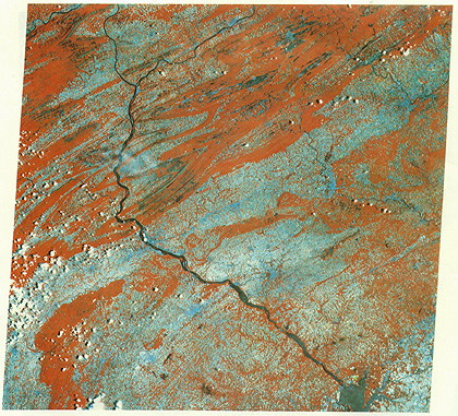
`**1-8:** <>`__ **Now examine the full MSS false color image of this region as seen on June 8, 1977. Account for the large areas in blue. Take note of the dark grayish-black patches on some of the ridges; there are also some blackish area in the valleys between ridges, primarily in the upper third of the image. We will take note of these special features later in this exam. Note the course of the Susquehanna River in the lower third of the image. At several places the river widens noticeably. Can you explain this. ANSWER **
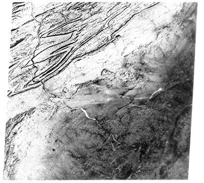
`**1-9:** <>`__ **Below is a scene taken on July 14, 1977. Describe the principal difference between this and the June 8th image. Look also in the vicinity of Harrisburg at the Susquehanna River. It is marked by a blue color on its left side; why? ANSWER **
`**1-10:** <>`__ **A Landsat 2 MSS Band 5 scene, taken on January 23, 1979, is reproduced below. Comment on differences you note in this image from those we've examined before. How might one distinguish snow from clouds? ANSWER **
在这一点上,我们将集中在哈里斯堡周围的一个单一的局部区域,以便更好地了解陆地卫星MSS图像中可以提取的细节(对于分辨率高出2倍以上的陆地卫星TM图像,会更清晰,但作者无法获得TM图像)。
但是,首先,要近距离地站起来,看看从哈里斯堡市中心东北方向的I-83大桥拍摄的地面场景。这座桥有一条铁路穿过苏斯奎汉纳河。在最左边的天际线是蓝山的一部分,也是河流流过的水隙。
1974年2月5日,我们在RB-57的下海湾安装了一台摄像机,从5万英尺高空拍摄了一张假彩色航空照片(比例尺1:142000)。
`**1-11:** <>`__ **Peruse this image. Locate Harrisburg first, then using an Atlas pinpoint other towns, major roadways, and the meandering (curving) river. Mention anything else you find interesting. ANSWER **
`**1-12:** <>`__**Knowing that the standard Landsat full scene (7.25 inches wide at its base, representing 115 miles across) has a scale of 1:1,000,000, calculate the width in miles of this aerial photo scene. ANSWER **
下面是1972年10月11日陆地卫星MSS假彩色合成图的一个次新世,它被放大到和上面的RB-57场景差不多的比例。它变得更蓝,看起来更像航空照片。
`**1-13:** <>`__ **Compare this subscene with the RB-57 photo, noting what can be found in both and what is not "seeable" in the Landsat version. ANSWER **
另外一个哈里斯堡次新统是1977年7月的假彩色合成。
`**1-14:** <>`__ **Comment on anything unusual or different in the above image. ANSWER **
现在我们将更仔细地观察放大图中的细节,集中在马里兰州埃尔克顿南部切萨皮克和特拉华运河周围的区域(这是1972年10月场景的右下角)。以下两幅图像中的第一幅是1977年7月图像集第5波段的512 x 512像素次新图像。下面是一张比例为1:60000的航空照片,包含陆地卫星图像中的农田;这张照片拍摄于同年5月。
`**1-15:** <>`__ **Can you locate the aerial photo in the Landsat subscene? Watch out - the field patterns have changed between the two dates for an obvious reason. ANSWER **
我们已经准备好改变方向,专注于像照片一样的自然图像的主要使用:变化检测。我们将使用从我们已经遇到的完整图像的上半部分切下的几个子场景。首先考虑一下这个:1977年6月8日的7级图像。
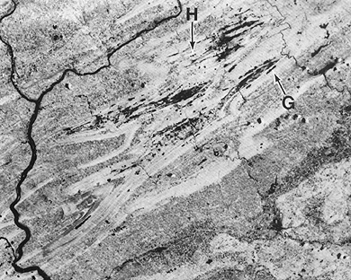
`**1-16:** <>`__ **One thing that is obvious: widespread patches of almost black features, found almost entirely in valleys between ridges. Do you have any idea what these represent? Hint: they are related to a geological material that has immense commercial value; this material is in beds in rocks of Pennsylvanian age. ANSWER **
`**1-17:** <>`__ **There are dark patterns, one elongate, the other as three spots, near the tips of arrows G and H. What do you think these are? Can you find them in corresponding local areas in the October 1972 MSS Band 7 image? What's going on? ANSWER **
下面是1973年7月8日刚刚看到的同一地区的mss 7次新世。
`**1-18:** <>`__ **What's new and different? Identify the features at arrow tips of the letters indicated (the rightmost arrow is labelled "I"). Features such as at "K" are a new phenomenon, in which the ground is responsible for the reflectance that gives rise to a medium gray tone (that's a clue!) ANSWER **
1977年,宾夕法尼亚州再次受到“K”现象的严重打击。下一幅插图是从宾夕法尼亚州威廉姆斯波特以北的一个地区(就在我们所看到的整个场景之外)拍摄的六个次新世面板。现在,不要看两个面板行之间的黑色打印。
`**1-19:** <>`__ **Since you now know what "K" is from the previous question, comment on the progression of the feature that appears gray-brown in these panels. ANSWER **
现在,我们将进入第二阶段的提问,在第二阶段中,你将被要求分析和评论在宾夕法尼亚州中南部的这项研究中产生的一些计算机生成的图像。
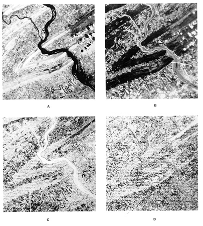
首先,是一个区域的四个次中心的一个小组,包括汉诺威,PA(在水库的左边,西部),大约20英里以南,宾夕法尼亚州约克西南。斜穿过每个次新世是一系列几乎平行的直线。在大多数完整场景中也可以看到这些。它们是由前寒武纪变质杂岩中抵抗力更强的单元雕刻而成的低脊,构成了山前的这一部分。场景如下:
左上角的图像是1978年6月场景的MSS波段7再现(拉伸);右下角是1978年2月场景的波段7的线性拉伸,其中地面被雪覆盖。右上角由六月次新世快速傅立叶变换的高带通滤波器组成,而左下角也是带5的高带通滤波器版本,带有三次卷积重采样。
`**1-20:** <>`__ **Which of the four subscenes seems best/worst for picking out linear features? Compare the Fast Fourier and Cubic Convolution processing for enhancing linear features and sharpening details. Make a guess as to the identity (nature) of the irregular feature (in medium to dark gray) that lies just south of the reservoir lake.ANSWER **
现在,回到哈里斯堡和吉普赛蛾的落叶。看看这个1977年6月27日的次新世。落叶在山脊上呈深灰色斑块。
在忽略图像中的其他功能/类的同时,有几种方法可以将注意力集中在这种落叶上。一种是计算图像的植被指数。对于这个vi,至少提出了六种不同的公式。我们将使用最简单的公式,即mss7/mss5的比率。完成此操作后,将出现一系列可以显示为灰色级别的DNS。但是,另一种方法是产生一个彩色蒙版图像。所有非植被特征设置为一个单一的dn值(将其掩盖),具有树木和森林特征的植被区域被赋予不同的颜色。这就是结果,遮蔽区域显示为黄灰色,健康森林显示为绿色,落叶森林显示为红色,强调植被为紫色。
`**1-21:** <>`__ **What is the advantage of this VI image? Where may confusion occur? ANSWER **
同一场景(和日期)已接受主要成分分析。前四个组件的图像如下所示(但在布局错误的情况下,第一个组件是B,第二个组件是A,C和D分别是第三个和第四个组件。
`**1-22:** <>`__ **Describe the main gray patterns in each component image. ANSWER **
颜色合成可以由这三个图像中的任何一个组成。一般来说,第四组分图像是平淡和模糊的,不使用。下面是使用pc 2=红色;pc 1=绿色;pc 3=蓝色制作的假彩色图像。
`**1-23:** <>`__ **What does this PC image show that is less obvious in the standard false color composite shown above?ANSWER **
我们现在准备开始在1972年10月的原始完整的MSS场景中对4个区域进行监督分类,我们在测试开始时已经对这些区域进行了检查。我们将从哈里斯堡次新世的8级地图开始。这以及随后的分类都是在NASA戈达德的IDims计算机系统上完成的。
`**1-24:** <>`__ **Evaluate this classification. ANSWER **
一直到无烟煤带。首先,我们提出了一个标准的次新世假彩色合成图,显示了哈兹尔顿(T)东南部从蓝山(最低的N)到大峡谷农业用地(A)的褶皱山脊。最亮的蓝色是我的废物。1973年7月8日的这一场景中,落叶较为温和,以蓝灰色为代表。
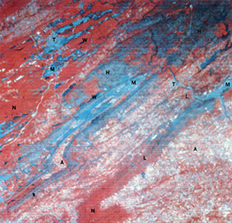
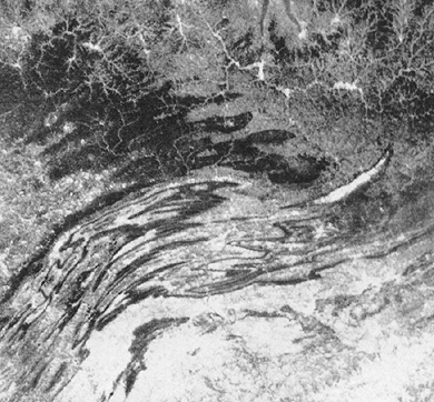
一张1:78000比例的黑白航空照片覆盖了部分陆地卫星次新世。
`**1-25:** <>`__**Try to fit this aerial photo into the Landsat scene. Name the towns (use Atlas) you find. Is the mine refuse well displayed in the photo. ANSWER **
让我们展望第16节,其中介绍了Terra航天器的产品。其中一个传感器,misr,已经产生了宾夕法尼亚州和纽约新泽西州东部地区的近自然色图像。
`**1-26:** <>`__**Is there anything special about the areas in the coal country we have been looking at? Why is this speciality ambiguous?ANSWER **
1973年7月8日在通用电子图像-100交互处理系统上对哈兹尔顿附近的次新世进行了无监督分类。只指定了四个集群类。当他们被屏蔽为模式后,他们就被命名,使用作者对该地区的一般知识。这里是:
`**1-27:** <>`__ **Evaluate this classification, compared with your expectations from the fcc image for this date. Use the lakes (shown in black) to relate the class map to the image. ANSWER **
接下来的两个分类处理了切萨皮克和特拉华运河周围的区域和切萨皮克湾源头,它们占据了1972年10月图像的右下角。
第一个是从1977年7月的完整场景中提取的次新世的监督分类(右),如下图所示,为假彩色图像。这些课程是作者在实地考察后选择的,并与当地的土壤保护服务代表进行了讨论。
`**1-28:** <>`__ **Which seems more abundant, corn or soybeans? If you consult a map of the area, you might conclude that most of the larger lavender patterns associate with towns and villages. But what about smaller clusters of lavender; what might they be? Give a reason why so many of the fields do not have straight boundaries, as is typical, nor are rectangular. ANSWER **
最后一个分类显示了马里兰州北部哈弗德格拉斯和阿伯丁附近切萨皮克湾源头的水纯度类别。图像采集日期为1978年5月28日。结果是:
萨斯奎汉纳河的河口位于中心顶部。切萨皮克湾本身就是下苏斯奎汉纳河的淹死部分,该河曾在弗吉尼亚州诺福克附近清空,但在最后一次冰川退却后被上升的海平面淹没。这里的土地通过遮罩被渲染为黑色(白色湿地除外),遮罩涉及将所有土地像素分配给一个单一的值(给定颜色)。
`**1-29:** <>`__ **How do you think the turbidity in the Bush River was determined (assessed)? ANSWER **
我们的“考试”快结束了。现在,我们将注意力转向另外两种类型的遥感器——那些产生主动微波的遥感器——雷达图像和那些测量热特性的遥感器。这些传感器系统分别在第8节和第9节中介绍。以下只是预览。
对于覆盖宾夕法尼亚地区和一些邻近州的热成像,我们将求助于名为HCMM(热容测绘任务;见第9节)的卫星。这项技术在1978年投入使用,并以三种模式制作了700公里宽的场景:白天可见、白天(热)红外和夜间红外。
首先看一天的红外图像(1978年9月26日),图像的下半部分包括我们一直在研究的哈里斯堡周围的大部分地区。暗色调对应“冷”;浅色对应“暖”。
`**1-30:** <>`__**First locate yourself within this image relative to the landmarks you have come to know. Why are the ridges cool (dark) and the valleys warm (light-toned)? There is a long, canoe-shaped white area in the right center; why does it appear to be so hot? While it is not in the region you have been studying, speculate on the very dark patterns in the upper center. ANSWER **
然后,看看这张1978年6月11日拍摄的夜间红外图像。
`**1-31:** <>`__ **Why do the ridges and rivers and other water bodies appear to be warmer (lighter toned) than the valleys? Can you find the Harrisburg area? ANSWER **
最后,我们在包括哈里斯堡地区在内的两幅雷达图像上拍摄一个短暂的峰值。由于雷达图像的解释需要对传感器的工作方式和图像的形成有相当的了解(我们将在第8节中详细了解),因此我们只向您展示两个示例。我们建议您在陆地卫星场景的框架中定位这些图像,并挑选出您已经熟悉的任何特殊特征和地标。第一张图片是由一个飞机安装的斯拉尔系统(K波段),因为它在1966年7月22日飞越地形。第二个是1978年9月28日由SEASAT SAR(L波段)从太空拍摄的。在这幅图像中,哈里斯堡的位置应该是显而易见的(它的建筑是很强的反射镜)。
`**1-32:** <>`__ **Compare the aircraft SLAR image with the Seasat image. Make note of any obvious differences between the two and suggest reason(s) why.ANSWER **
好吧,我们的“考试”到此结束。相当有挑战性,但希望不是乏味。给自己打分,但仅仅通过努力,你就应该得到“A”。在本教程的其余部分中,在期末考试(第21节)之前,我们将不再面临如此广泛的问题序列,但在这两个部分之间的几乎所有部分中,都将有足够的查询来帮助您更好地了解与远程操作相关的重要概念和功能。感知解释。
点击 here 回到第一节的最后一页。