4.2. 轮廓特征
4.2.2. 一。瞬间
图像矩可以帮助您计算一些特征,如物体的质心、面积等。请查看 Image Moments
函数 cv2.力矩() 提供计算的所有力矩值的字典。见下文:
>>> %matplotlib inline
>>> import matplotlib.pyplot as plt
>>>
>>> import cv2
>>> import numpy as np
>>>
>>> # img = cv2.imread('/cvdata/star.jpg',0)
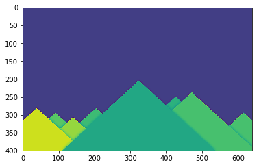
>>> img = cv2.imread('/cvdata/star.png', 0)
>>> plt.imshow(img)
<matplotlib.image.AxesImage at 0x7f2aec184cc0>
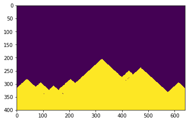
>>> ret,thresh = cv2.threshold(img,127,255,0)
>>> ret
127.0
>>> plt.imshow(thresh)
<matplotlib.image.AxesImage at 0x7f2aec0e7780>
>>> contours,hierarchy,aa = cv2.findContours(thresh, 1, 2)
>>> contours.shape
(400, 640)
>>> aa.shape
(1, 22, 4)
>>> cnt = contours[0]
>>> M = cv2.moments(cnt)
>>> print (M)
{'m00': 0.0, 'm10': 0.0, 'm01': 0.0, 'm20': 0.0, 'm11': 0.0, 'm02': 0.0, 'm30': 0.0, 'm21': 0.0, 'm12': 0.0, 'm03': 0.0, 'mu20': 0.0, 'mu11': 0.0, 'mu02': 0.0, 'mu30': 0.0, 'mu21': 0.0, 'mu12': 0.0, 'mu03': 0.0, 'nu20': 0.0, 'nu11': 0.0, 'nu02': 0.0, 'nu30': 0.0, 'nu21': 0.0, 'nu12': 0.0, 'nu03': 0.0}
从这个时刻,你可以提取有用的数据,如面积,质心等。质心由关系给出, \(C_x = \frac{{M_{{10}}}}{{M_{{00}}}}\) 和 \(C_y = \frac{{M_{{01}}}}{{M_{{00}}}}\) . 具体操作如下:
>>> cx = int(M['m10']/M['m00'])
>>> cy = int(M['m01']/M['m00'])
---------------------------------------------------------------------------

ZeroDivisionError                         Traceback (most recent call last)

<ipython-input-78-6f707285d91a> in <module>()
----> 1 cx = int(M['m10']/M['m00'])
      2 cy = int(M['m01']/M['m00'])


ZeroDivisionError: float division by zero
4.2.3. 2。等高线面积
轮廓面积由函数给出 等高线面积() 或者从某个时刻开始, [M[‘m00’]] .
>>> for x in hierarchy:
>>>     area = cv2.contourArea(x)
>>>     print(area)
4.0
4.0
2.0
2.0
8.5
2.0
2.0
2.0
2.0
2.0
2.0
2.0
2.0
2.0
2.0
2.0
2.0
2.0
2.0
2.0
2.0
76185.5
4.2.4. 三。等高线周长
也称为弧长。你可以用 弧长() 功能。第二个参数指定形状是否为闭合轮廓(如果传递 True ),或者只是曲线。
>>> for cnt in hierarchy:
>>>     perimeter = cv2.arcLength(cnt,True)
>>>     print(perimeter)
7.656854152679443
7.656854152679443
5.656854152679443
5.656854152679443
11.071067690849304
5.656854152679443
5.656854152679443
5.656854152679443
5.656854152679443
5.656854152679443
5.656854152679443
5.656854152679443
5.656854152679443
5.656854152679443
5.656854152679443
5.656854152679443
5.656854152679443
5.656854152679443
5.656854152679443
5.656854152679443
5.656854152679443
1680.687520623207
4.2.5. 四。轮廓近似
根据我们指定的精度,它将一个轮廓形状近似为另一个顶点数较少的形状。它是 Douglas-Peucker algorithm . 查看维基百科页面上的算法和演示。
为了理解这一点,假设您试图在图像中找到一个正方形,但是由于图像中的一些问题,您没有得到一个完美的正方形,而是得到了一个“坏形状”(如下图所示)。现在可以使用此函数来近似形状。在这里,第二个参数被称为 epsilon ,这是从轮廓到近似轮廓的最大距离。它是一个精度参数。明智的选择 epsilon 需要得到正确的输出。
>>> for cnt in hierarchy:
>>>     epsilon = 0.1*cv2.arcLength(cnt,True)
>>>     approx = cv2.approxPolyDP(cnt,epsilon,True)
>>>     print(epsilon, approx)
0.7656854152679444 [[[175 338]]

 [[176 337]]

 [[178 338]]

 [[177 339]]]
0.7656854152679444 [[[102 338]]

 [[103 337]]

 [[105 338]]

 [[104 339]]]
0.5656854152679444 [[[174 337]]

 [[175 336]]

 [[176 337]]

 [[175 338]]]
0.5656854152679444 [[[173 336]]

 [[174 335]]

 [[175 336]]

 [[174 337]]]
1.1071067690849306 [[[413 286]]

 [[416 285]]

 [[417 287]]

 [[415 288]]]
0.5656854152679444 [[[416 285]]

 [[417 284]]

 [[418 285]]

 [[417 286]]]
0.5656854152679444 [[[412 285]]

 [[413 284]]

 [[414 285]]

 [[413 286]]]
0.5656854152679444 [[[417 284]]

 [[418 283]]

 [[419 284]]

 [[418 285]]]
0.5656854152679444 [[[411 284]]

 [[412 283]]

 [[413 284]]

 [[412 285]]]
0.5656854152679444 [[[421 281]]

 [[422 280]]

 [[423 281]]

 [[422 282]]]
0.5656854152679444 [[[422 280]]

 [[423 279]]

 [[424 280]]

 [[423 281]]]
0.5656854152679444 [[[423 279]]

 [[424 278]]

 [[425 279]]

 [[424 280]]]
0.5656854152679444 [[[424 278]]

 [[425 277]]

 [[426 278]]

 [[425 279]]]
0.5656854152679444 [[[425 277]]

 [[426 276]]

 [[427 277]]

 [[426 278]]]
0.5656854152679444 [[[426 276]]

 [[427 275]]

 [[428 276]]

 [[427 277]]]
0.5656854152679444 [[[431 272]]

 [[432 271]]

 [[433 272]]

 [[432 273]]]
0.5656854152679444 [[[432 271]]

 [[433 270]]

 [[434 271]]

 [[433 272]]]
0.5656854152679444 [[[433 270]]

 [[434 269]]

 [[435 270]]

 [[434 271]]]
0.5656854152679444 [[[434 269]]

 [[435 268]]

 [[436 269]]

 [[435 270]]]
0.5656854152679444 [[[435 268]]

 [[436 267]]

 [[437 268]]

 [[436 269]]]
0.5656854152679444 [[[436 267]]

 [[437 266]]

 [[438 267]]

 [[437 268]]]
168.06875206232073 [[[639 316]]

 [[  0 399]]]
下图中,绿线显示了 epsilon = 10% of arc length . 第三张图片显示了相同的 epsilon = 1% of the arc length . 第三个参数指定曲线是否闭合。
4.2.6. 5个。凸壳
凸包看起来类似于轮廓近似,但它不是(在某些情况下两者可能提供相同的结果)。在这里, cv2.对流式() 函数检查曲线是否存在凸性缺陷并对其进行更正。一般来说,凸曲线是指曲线总是凸出,或者至少是平坦的。如果它在内部膨胀,称为凸缺陷。例如,检查下面的手的图像。红线表示手的凸面外壳。双面箭头标记显示了船体的凸度缺陷,即船体与轮廓线的局部最大偏差。
关于它的语法有一点需要讨论:
>>> hull = cv2.convexHull(points[, hull[, clockwise[, returnPoints]]
参数详细信息:
点 是我们穿过的轮廓。
hull 是输出,通常我们会避免它。
顺时针方向的 :方向标志。如果是的话
True,输出凸包为顺时针方向。否则,它是逆时针方向的。返回点 :默认情况下,
True. 然后返回外壳点的坐标。如果False,它返回与外壳点相对应的轮廓点的索引。
因此,要获得如上图所示的凸面外壳,以下内容就足够了:
>>> hull = cv2.convexHull(cnt)
但是如果你想找到凸性缺陷,你需要通过 returnPoints = False . 为了理解它,我们将拍摄上面的矩形图像。首先我发现它的轮廓是 cnt . 现在我发现它的凸面外壳 returnPoints = True ,我得到了以下值: [[[234 202]], [[ 51 202]], [[ 51 79]], [[234 79]]] 这是矩形的四个角点。如果你也这么做 returnPoints = False ,得到以下结果: [[129],[ 67],[ 0],[142]] . 这些是等高线中对应点的索引。例如,检查第一个值: cnt[129] = [[234, 202]] 这和第一个结果是一样的(对其他人也是如此)。
当我们讨论凸性缺陷时,你们会再次看到它。
4.2.7. 6。检查凸性
有一个函数可以检查曲线是否是凸的, cv2.isContourConvex() . 不管是真是假,它都会返回。没什么大不了的。
>>> k = cv2.isContourConvex(cnt)
4.2.8. 7号。边界矩形
有两种类型的边界矩形。
7.a.直边矩形
它是一个直矩形,不考虑对象的旋转。所以边界矩形的面积不会是最小的。它是由函数找到的 cv2.boundingRect() .
设(x,y)为矩形的左上角坐标,(w,h)为矩形的宽度和高度。
>>> x,y,w,h = cv2.boundingRect(cnt)
>>> img = cv2.rectangle(img,(x,y),(x+w,y+h),(0,255,0),2)
7.b.旋转矩形
在这里,边界矩形是用最小面积绘制的,所以它也考虑了旋转。使用的函数是 化学气相色谱仪 . 它返回一个Box2D结构,包含以下细节(左上角(x,y),(宽度,高度),旋转角度)。但是要画这个矩形,我们需要矩形的四个角。它是通过函数得到的 箱形点()
>>> rect = cv2.minAreaRect(cnt)
>>> box = cv2.boxPoints(rect)
>>> box = np.int0(box)
>>> im = cv2.drawContours(img,[box],0,(0,0,255),2)
>>> plt.imshow(im)
<matplotlib.image.AxesImage at 0x7f2aec05f2b0>
两个矩形都显示在一个图像中。绿色矩形显示法向边界矩形。红色矩形是旋转的矩形。
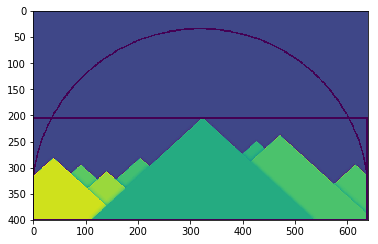
4.2.9. 8个。最小包围圈
接下来我们用函数求出一个物体的外圆 cv2.minEnclosingCircle() . 它是一个完全覆盖物体最小面积的圆。
>>> (x,y),radius = cv2.minEnclosingCircle(cnt)
>>> center = (int(x),int(y))
>>> radius = int(radius)
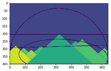
>>> img = cv2.circle(img,center,radius,(0,255,0),2)
>>> plt.imshow(img)
<matplotlib.image.AxesImage at 0x7f2aec032f98>
4.2.10. 9号。拟合椭圆
下一步是将椭圆拟合到对象上。它返回椭圆内接的旋转矩形。
>>> ellipse = cv2.fitEllipse(cnt)
>>> im = cv2.ellipse(im,ellipse,(0,255,0),2)
>>> plt.imshow(im)
<matplotlib.image.AxesImage at 0x7f2ae677dc50>

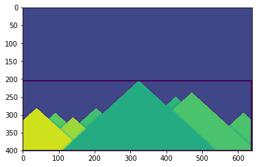
4.2.11. 10个。装线
同样,我们可以将一条直线拟合到一组点上。下图包含一组白点。我们可以把它近似成一条直线。
>>> rows,cols = img.shape[:2]
>>> [vx,vy,x,y] = cv2.fitLine(cnt, cv2.DIST_L2,0,0.01,0.01)
>>> lefty = int((-x*vy/vx) + y)
>>> righty = int(((cols-x)*vy/vx)+y)
>>> img = cv2.line(img,(cols-1,righty),(0,lefty),(0,255,0),2)
>>> plt.imshow(img)
<matplotlib.image.AxesImage at 0x7f2ae67648d0>