注释绘图

以下示例说明如何在Matplotlib中注释打印。这包括突出显示特定的兴趣点，并使用各种视觉工具来引起对这一点的注意。有关Matplotlib中注释和文本工具的更完整和更深入的说明，请参见 tutorial on annotation .

import matplotlib.pyplot as plt
from matplotlib.patches import Ellipse
import numpy as np
from matplotlib.text import OffsetFrom

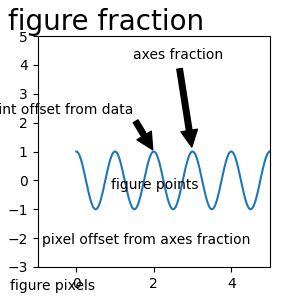
指定文本点和注释点

必须指定批注点 xy=(x, y) 来诠释这一点。此外，还可以指定文本点 xytext=(x, y) 用于此批注的文本位置。或者，可以指定 xy 和 木文 使用以下字符串之一 木栓 和 文本框 （默认为“数据”）：：

'figure points'   : points from the lower left corner of the figure
'figure pixels'   : pixels from the lower left corner of the figure
'figure fraction' : (0, 0) is lower left of figure and (1, 1) is upper right
'axes points'     : points from lower left corner of axes
'axes pixels'     : pixels from lower left corner of axes
'axes fraction'   : (0, 0) is lower left of axes and (1, 1) is upper right
'offset points'   : Specify an offset (in points) from the xy value
'offset pixels'   : Specify an offset (in pixels) from the xy value
'data'            : use the axes data coordinate system

注：对于物理坐标系（点或像素），原点是图形或轴的（底部、左侧）。

或者，通过提供箭头属性字典，可以指定从文本到带注释点的箭头属性，并从文本到带注释点进行绘制和箭头。

有效密钥为：

width : the width of the arrow in points
frac  : the fraction of the arrow length occupied by the head
headwidth : the width of the base of the arrow head in points
shrink : move the tip and base some percent away from the
         annotated point and text
any key for matplotlib.patches.polygon  (e.g., facecolor)

# Create our figure and data we'll use for plotting
fig, ax = plt.subplots(figsize=(3, 3))

t = np.arange(0.0, 5.0, 0.01)
s = np.cos(2*np.pi*t)

# Plot a line and add some simple annotations
line, = ax.plot(t, s)
ax.annotate('figure pixels',
            xy=(10, 10), xycoords='figure pixels')
ax.annotate('figure points',
            xy=(80, 80), xycoords='figure points')
ax.annotate('figure fraction',
            xy=(.025, .975), xycoords='figure fraction',
            horizontalalignment='left', verticalalignment='top',
            fontsize=20)

# The following examples show off how these arrows are drawn.

ax.annotate('point offset from data',
            xy=(2, 1), xycoords='data',
            xytext=(-15, 25), textcoords='offset points',
            arrowprops=dict(facecolor='black', shrink=0.05),
            horizontalalignment='right', verticalalignment='bottom')

ax.annotate('axes fraction',
            xy=(3, 1), xycoords='data',
            xytext=(0.8, 0.95), textcoords='axes fraction',
            arrowprops=dict(facecolor='black', shrink=0.05),
            horizontalalignment='right', verticalalignment='top')

# You may also use negative points or pixels to specify from (right, top).
# E.g., (-10, 10) is 10 points to the left of the right side of the axes and 10
# points above the bottom

ax.annotate('pixel offset from axes fraction',
            xy=(1, 0), xycoords='axes fraction',
            xytext=(-20, 20), textcoords='offset pixels',
            horizontalalignment='right',
            verticalalignment='bottom')

ax.set(xlim=(-1, 5), ylim=(-3, 5))

出：

[(-1.0, 5.0), (-3.0, 5.0)]

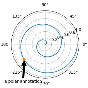
使用多个坐标系和轴类型

您可以指定 xypoint公司 以及 木文 在不同的位置和坐标系中，并可选地打开连接线并用标记标记标记该点。注释也适用于极轴。

在下面的示例中， xy 点在本机坐标系中( 木栓 默认为“数据”）。对于极轴，这是在（θ，半径）空间中。示例中的文本放置在分数图形坐标系中。文本关键字参数，如水平和垂直对齐。

fig, ax = plt.subplots(subplot_kw=dict(projection='polar'), figsize=(3, 3))
r = np.arange(0, 1, 0.001)
theta = 2*2*np.pi*r
line, = ax.plot(theta, r)

ind = 800
thisr, thistheta = r[ind], theta[ind]
ax.plot([thistheta], [thisr], 'o')
ax.annotate('a polar annotation',
            xy=(thistheta, thisr),  # theta, radius
            xytext=(0.05, 0.05),    # fraction, fraction
            textcoords='figure fraction',
            arrowprops=dict(facecolor='black', shrink=0.05),
            horizontalalignment='left',
            verticalalignment='bottom')

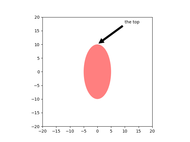
# You can also use polar notation on a cartesian axes.  Here the native
# coordinate system ('data') is cartesian, so you need to specify the
# xycoords and textcoords as 'polar' if you want to use (theta, radius).

el = Ellipse((0, 0), 10, 20, facecolor='r', alpha=0.5)

fig, ax = plt.subplots(subplot_kw=dict(aspect='equal'))
ax.add_artist(el)
el.set_clip_box(ax.bbox)
ax.annotate('the top',
            xy=(np.pi/2., 10.),      # theta, radius
            xytext=(np.pi/3, 20.),   # theta, radius
            xycoords='polar',
            textcoords='polar',
            arrowprops=dict(facecolor='black', shrink=0.05),
            horizontalalignment='left',
            verticalalignment='bottom',
            clip_on=True)  # clip to the axes bounding box

ax.set(xlim=[-20, 20], ylim=[-20, 20])

• 
• 

出：

[(-20.0, 20.0), (-20.0, 20.0)]

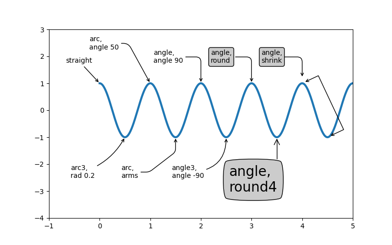
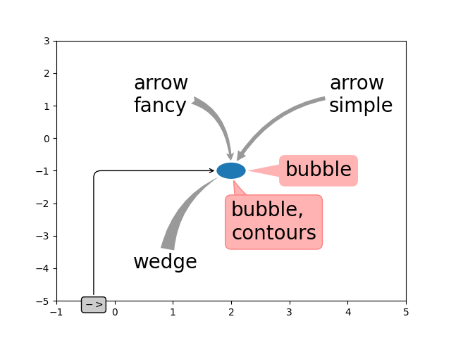
自定义箭头和气泡样式

之间的箭头 木文 注释点以及覆盖注释文本的气泡都是高度可定制的。下面是一些参数选项及其结果输出。

fig, ax = plt.subplots(figsize=(8, 5))

t = np.arange(0.0, 5.0, 0.01)
s = np.cos(2*np.pi*t)
line, = ax.plot(t, s, lw=3)

ax.annotate(
    'straight',
    xy=(0, 1), xycoords='data',
    xytext=(-50, 30), textcoords='offset points',
    arrowprops=dict(arrowstyle="->"))
ax.annotate(
    'arc3,\nrad 0.2',
    xy=(0.5, -1), xycoords='data',
    xytext=(-80, -60), textcoords='offset points',
    arrowprops=dict(arrowstyle="->",
                    connectionstyle="arc3,rad=.2"))
ax.annotate(
    'arc,\nangle 50',
    xy=(1., 1), xycoords='data',
    xytext=(-90, 50), textcoords='offset points',
    arrowprops=dict(arrowstyle="->",
                    connectionstyle="arc,angleA=0,armA=50,rad=10"))
ax.annotate(
    'arc,\narms',
    xy=(1.5, -1), xycoords='data',
    xytext=(-80, -60), textcoords='offset points',
    arrowprops=dict(
        arrowstyle="->",
        connectionstyle="arc,angleA=0,armA=40,angleB=-90,armB=30,rad=7"))
ax.annotate(
    'angle,\nangle 90',
    xy=(2., 1), xycoords='data',
    xytext=(-70, 30), textcoords='offset points',
    arrowprops=dict(arrowstyle="->",
                    connectionstyle="angle,angleA=0,angleB=90,rad=10"))
ax.annotate(
    'angle3,\nangle -90',
    xy=(2.5, -1), xycoords='data',
    xytext=(-80, -60), textcoords='offset points',
    arrowprops=dict(arrowstyle="->",
                    connectionstyle="angle3,angleA=0,angleB=-90"))
ax.annotate(
    'angle,\nround',
    xy=(3., 1), xycoords='data',
    xytext=(-60, 30), textcoords='offset points',
    bbox=dict(boxstyle="round", fc="0.8"),
    arrowprops=dict(arrowstyle="->",
                    connectionstyle="angle,angleA=0,angleB=90,rad=10"))
ax.annotate(
    'angle,\nround4',
    xy=(3.5, -1), xycoords='data',
    xytext=(-70, -80), textcoords='offset points',
    size=20,
    bbox=dict(boxstyle="round4,pad=.5", fc="0.8"),
    arrowprops=dict(arrowstyle="->",
                    connectionstyle="angle,angleA=0,angleB=-90,rad=10"))
ax.annotate(
    'angle,\nshrink',
    xy=(4., 1), xycoords='data',
    xytext=(-60, 30), textcoords='offset points',
    bbox=dict(boxstyle="round", fc="0.8"),
    arrowprops=dict(arrowstyle="->",
                    shrinkA=0, shrinkB=10,
                    connectionstyle="angle,angleA=0,angleB=90,rad=10"))
# You can pass an empty string to get only annotation arrows rendered
ax.annotate('', xy=(4., 1.), xycoords='data',
            xytext=(4.5, -1), textcoords='data',
            arrowprops=dict(arrowstyle="<->",
                            connectionstyle="bar",
                            ec="k",
                            shrinkA=5, shrinkB=5))

ax.set(xlim=(-1, 5), ylim=(-4, 3))

# We'll create another figure so that it doesn't get too cluttered
fig, ax = plt.subplots()

el = Ellipse((2, -1), 0.5, 0.5)
ax.add_patch(el)

ax.annotate('$->$',
            xy=(2., -1), xycoords='data',
            xytext=(-150, -140), textcoords='offset points',
            bbox=dict(boxstyle="round", fc="0.8"),
            arrowprops=dict(arrowstyle="->",
                            patchB=el,
                            connectionstyle="angle,angleA=90,angleB=0,rad=10"))
ax.annotate('arrow\nfancy',
            xy=(2., -1), xycoords='data',
            xytext=(-100, 60), textcoords='offset points',
            size=20,
            # bbox=dict(boxstyle="round", fc="0.8"),
            arrowprops=dict(arrowstyle="fancy",
                            fc="0.6", ec="none",
                            patchB=el,
                            connectionstyle="angle3,angleA=0,angleB=-90"))
ax.annotate('arrow\nsimple',
            xy=(2., -1), xycoords='data',
            xytext=(100, 60), textcoords='offset points',
            size=20,
            # bbox=dict(boxstyle="round", fc="0.8"),
            arrowprops=dict(arrowstyle="simple",
                            fc="0.6", ec="none",
                            patchB=el,
                            connectionstyle="arc3,rad=0.3"))
ax.annotate('wedge',
            xy=(2., -1), xycoords='data',
            xytext=(-100, -100), textcoords='offset points',
            size=20,
            # bbox=dict(boxstyle="round", fc="0.8"),
            arrowprops=dict(arrowstyle="wedge,tail_width=0.7",
                            fc="0.6", ec="none",
                            patchB=el,
                            connectionstyle="arc3,rad=-0.3"))
ax.annotate('bubble,\ncontours',
            xy=(2., -1), xycoords='data',
            xytext=(0, -70), textcoords='offset points',
            size=20,
            bbox=dict(boxstyle="round",
                      fc=(1.0, 0.7, 0.7),
                      ec=(1., .5, .5)),
            arrowprops=dict(arrowstyle="wedge,tail_width=1.",
                            fc=(1.0, 0.7, 0.7), ec=(1., .5, .5),
                            patchA=None,
                            patchB=el,
                            relpos=(0.2, 0.8),
                            connectionstyle="arc3,rad=-0.1"))
ax.annotate('bubble',
            xy=(2., -1), xycoords='data',
            xytext=(55, 0), textcoords='offset points',
            size=20, va="center",
            bbox=dict(boxstyle="round", fc=(1.0, 0.7, 0.7), ec="none"),
            arrowprops=dict(arrowstyle="wedge,tail_width=1.",
                            fc=(1.0, 0.7, 0.7), ec="none",
                            patchA=None,
                            patchB=el,
                            relpos=(0.2, 0.5)))

ax.set(xlim=(-1, 5), ylim=(-5, 3))

• 
• 

出：

[(-1.0, 5.0), (-5.0, 3.0)]

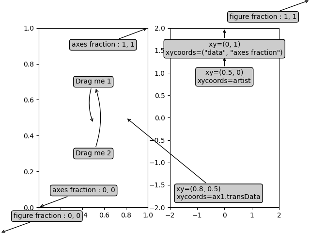
坐标系的更多示例

下面我们将展示更多关于坐标系的例子，以及如何指定注释的位置。

fig, (ax1, ax2) = plt.subplots(1, 2)

bbox_args = dict(boxstyle="round", fc="0.8")
arrow_args = dict(arrowstyle="->")

# Here we'll demonstrate the extents of the coordinate system and how
# we place annotating text.

ax1.annotate('figure fraction : 0, 0', xy=(0, 0), xycoords='figure fraction',
             xytext=(20, 20), textcoords='offset points',
             ha="left", va="bottom",
             bbox=bbox_args,
             arrowprops=arrow_args)

ax1.annotate('figure fraction : 1, 1', xy=(1, 1), xycoords='figure fraction',
             xytext=(-20, -20), textcoords='offset points',
             ha="right", va="top",
             bbox=bbox_args,
             arrowprops=arrow_args)

ax1.annotate('axes fraction : 0, 0', xy=(0, 0), xycoords='axes fraction',
             xytext=(20, 20), textcoords='offset points',
             ha="left", va="bottom",
             bbox=bbox_args,
             arrowprops=arrow_args)

ax1.annotate('axes fraction : 1, 1', xy=(1, 1), xycoords='axes fraction',
             xytext=(-20, -20), textcoords='offset points',
             ha="right", va="top",
             bbox=bbox_args,
             arrowprops=arrow_args)

# It is also possible to generate draggable annotations

an1 = ax1.annotate('Drag me 1', xy=(.5, .7), xycoords='data',
                   #xytext=(.5, .7), textcoords='data',
                   ha="center", va="center",
                   bbox=bbox_args,
                   #arrowprops=arrow_args
                   )

an2 = ax1.annotate('Drag me 2', xy=(.5, .5), xycoords=an1,
                   xytext=(.5, .3), textcoords='axes fraction',
                   ha="center", va="center",
                   bbox=bbox_args,
                   arrowprops=dict(patchB=an1.get_bbox_patch(),
                                   connectionstyle="arc3,rad=0.2",
                                   **arrow_args))
an1.draggable()
an2.draggable()

an3 = ax1.annotate('', xy=(.5, .5), xycoords=an2,
                   xytext=(.5, .5), textcoords=an1,
                   ha="center", va="center",
                   bbox=bbox_args,
                   arrowprops=dict(patchA=an1.get_bbox_patch(),
                                   patchB=an2.get_bbox_patch(),
                                   connectionstyle="arc3,rad=0.2",
                                   **arrow_args))

# Finally we'll show off some more complex annotation and placement

text = ax2.annotate('xy=(0, 1)\nxycoords=("data", "axes fraction")',
                    xy=(0, 1), xycoords=("data", 'axes fraction'),
                    xytext=(0, -20), textcoords='offset points',
                    ha="center", va="top",
                    bbox=bbox_args,
                    arrowprops=arrow_args)

ax2.annotate('xy=(0.5, 0)\nxycoords=artist',
             xy=(0.5, 0.), xycoords=text,
             xytext=(0, -20), textcoords='offset points',
             ha="center", va="top",
             bbox=bbox_args,
             arrowprops=arrow_args)

ax2.annotate('xy=(0.8, 0.5)\nxycoords=ax1.transData',
             xy=(0.8, 0.5), xycoords=ax1.transData,
             xytext=(10, 10),
             textcoords=OffsetFrom(ax2.bbox, (0, 0), "points"),
             ha="left", va="bottom",
             bbox=bbox_args,
             arrowprops=arrow_args)

ax2.set(xlim=[-2, 2], ylim=[-2, 2])
plt.show()