使用Cartopy和matplotlib进行更高级的映射

从一开始，Cartopy的目的就是简化和提高科学数据可用的地图可视化质量。

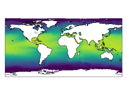
等高线图

import matplotlib.pyplot as plt
from scipy.io import netcdf

from cartopy import config
import cartopy.crs as ccrs


# get the path of the file. It can be found in the repo data directory.
fname = config["repo_data_dir"] / 'netcdf' / 'HadISST1_SST_update.nc'

dataset = netcdf.netcdf_file(fname, maskandscale=True, mmap=False)
sst = dataset.variables['sst'][0, :, :]
lats = dataset.variables['lat'][:]
lons = dataset.variables['lon'][:]

ax = plt.axes(projection=ccrs.PlateCarree())

plt.contourf(lons, lats, sst, 60,
             transform=ccrs.PlateCarree())

ax.coastlines()

plt.show()

(Source code)

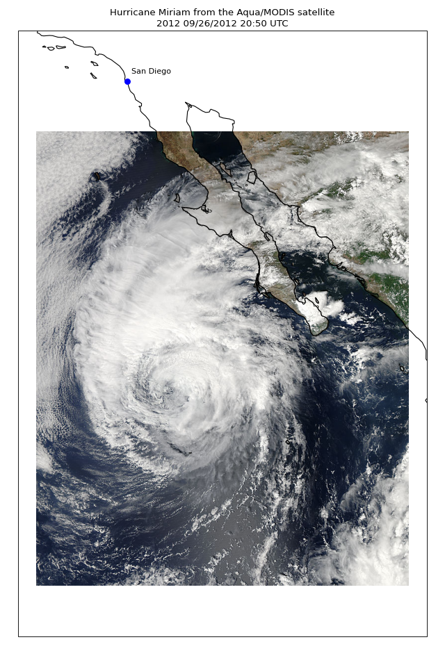
图像

import os
import matplotlib.pyplot as plt

from cartopy import config
import cartopy.crs as ccrs


fig = plt.figure(figsize=(8, 12))

# get the path of the file. It can be found in the repo data directory.
fname = config["repo_data_dir"] / 'raster' / 'sample' / 'Miriam.A2012270.2050.2km.jpg'
img_extent = (-120.67660000000001, -106.32104523100001, 13.2301484511245, 30.766899999999502)
img = plt.imread(fname)

ax = plt.axes(projection=ccrs.PlateCarree())
plt.title('Hurricane Miriam from the Aqua/MODIS satellite\n'
          '2012 09/26/2012 20:50 UTC')

ax.use_sticky_edges = False
# set a margin around the data
ax.set_xmargin(0.05)
ax.set_ymargin(0.10)

# add the image. Because this image was a tif, the "origin" of the image is in the
# upper left corner
ax.imshow(img, origin='upper', extent=img_extent, transform=ccrs.PlateCarree())
ax.coastlines(resolution='50m', color='black', linewidth=1)

# mark a known place to help us geo-locate ourselves
ax.plot(-117.1625, 32.715, 'bo', markersize=7, transform=ccrs.Geodetic())
ax.text(-117, 33, 'San Diego', transform=ccrs.Geodetic())

plt.show()

(Source code)

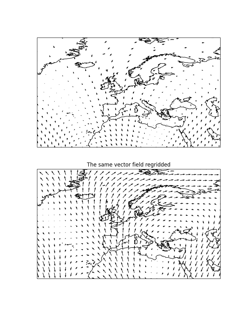
向图

Cartopy comes with powerful vector field plotting functionality. There are 3 distinct options for visualising vector fields: quivers (example), barbs (example) and streamplots (example) each with their own benefits for displaying certain vector field forms.

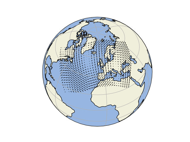
由于两 quiver() 和 barbs() 是绘制所提供的每个载体的可视化，还有一个额外的选项可以将载体场“重新网格化”到目标投影上的规则网格中（通过 cartopy.vector_transform.vector_scalar_to_grid() ).这是通过 regrid_shape 关键词，并且可能对可视化的有效性产生巨大影响：