绘制二维数据集的置信椭圆

这个例子展示了如何使用二维数据集的pearson相关系数绘制置信椭圆。

此处解释并证明了用于获得正确几何体的方法：

https://carstenschelp.github.io/2018/09/14/Plot_Confidence_Ellipse_001.html

该方法避免了迭代特征分解算法的使用，并利用了归一化协方差矩阵（由pearson相关系数和1组成）特别容易处理的事实。

import numpy as np
import matplotlib.pyplot as plt
from matplotlib.patches import Ellipse
import matplotlib.transforms as transforms

绘图功能本身

此函数绘制给定数组（如变量x和y）协方差的置信椭圆。椭圆被绘制到给定的轴对象ax中。

椭圆的半径可由标准偏差数n_std控制。默认值是3，这使得椭圆包含99.7%的点（假设数据像这些示例中一样是正态分布的）。

def confidence_ellipse(x, y, ax, n_std=3.0, facecolor='none', **kwargs):
    """
    Create a plot of the covariance confidence ellipse of *x* and *y*.

    Parameters
    ----------
    x, y : array-like, shape (n, )
        Input data.

    ax : matplotlib.axes.Axes
        The axes object to draw the ellipse into.

    n_std : float
        The number of standard deviations to determine the ellipse's radiuses.

    **kwargs
        Forwarded to `~matplotlib.patches.Ellipse`

    Returns
    -------
    matplotlib.patches.Ellipse
    """
    if x.size != y.size:
        raise ValueError("x and y must be the same size")

    cov = np.cov(x, y)
    pearson = cov[0, 1]/np.sqrt(cov[0, 0] * cov[1, 1])
    # Using a special case to obtain the eigenvalues of this
    # two-dimensionl dataset.
    ell_radius_x = np.sqrt(1 + pearson)
    ell_radius_y = np.sqrt(1 - pearson)
    ellipse = Ellipse((0, 0), width=ell_radius_x * 2, height=ell_radius_y * 2,
                      facecolor=facecolor, **kwargs)

    # Calculating the stdandard deviation of x from
    # the squareroot of the variance and multiplying
    # with the given number of standard deviations.
    scale_x = np.sqrt(cov[0, 0]) * n_std
    mean_x = np.mean(x)

    # calculating the stdandard deviation of y ...
    scale_y = np.sqrt(cov[1, 1]) * n_std
    mean_y = np.mean(y)

    transf = transforms.Affine2D() \
        .rotate_deg(45) \
        .scale(scale_x, scale_y) \
        .translate(mean_x, mean_y)

    ellipse.set_transform(transf + ax.transData)
    return ax.add_patch(ellipse)

创建相关数据集的帮助函数

使用指定的二维平均值（mu）和维度（scale）创建随机二维数据集。相关性可由参数“依赖性”控制，即2x2矩阵。

def get_correlated_dataset(n, dependency, mu, scale):
    latent = np.random.randn(n, 2)
    dependent = latent.dot(dependency)
    scaled = dependent * scale
    scaled_with_offset = scaled + mu
    # return x and y of the new, correlated dataset
    return scaled_with_offset[:, 0], scaled_with_offset[:, 1]

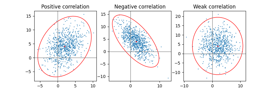
正、负、弱相关

注意，弱相关（右）的形状是椭圆，而不是圆，因为x和y的比例不同。然而，椭圆的轴与坐标系的x轴和y轴对齐，说明了x和y是不相关的。

np.random.seed(0)

PARAMETERS = {
    'Positive correlation': [[0.85, 0.35],
                             [0.15, -0.65]],
    'Negative correlation': [[0.9, -0.4],
                             [0.1, -0.6]],
    'Weak correlation': [[1, 0],
                         [0, 1]],
}

mu = 2, 4
scale = 3, 5

fig, axs = plt.subplots(1, 3, figsize=(9, 3))
for ax, (title, dependency) in zip(axs, PARAMETERS.items()):
    x, y = get_correlated_dataset(800, dependency, mu, scale)
    ax.scatter(x, y, s=0.5)

    ax.axvline(c='grey', lw=1)
    ax.axhline(c='grey', lw=1)

    confidence_ellipse(x, y, ax, edgecolor='red')

    ax.scatter(mu[0], mu[1], c='red', s=3)
    ax.set_title(title)

plt.show()

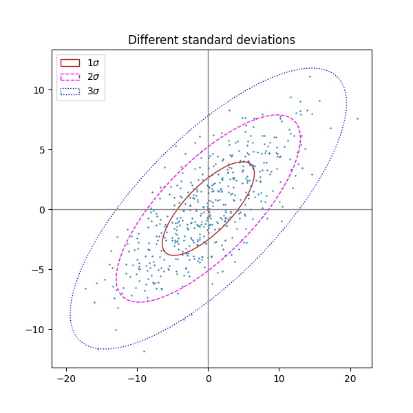
不同数量的标准差

n_std=3（蓝色）、2（紫色）和1（红色）的绘图

fig, ax_nstd = plt.subplots(figsize=(6, 6))

dependency_nstd = [[0.8, 0.75],
                   [-0.2, 0.35]]
mu = 0, 0
scale = 8, 5

ax_nstd.axvline(c='grey', lw=1)
ax_nstd.axhline(c='grey', lw=1)

x, y = get_correlated_dataset(500, dependency_nstd, mu, scale)
ax_nstd.scatter(x, y, s=0.5)

confidence_ellipse(x, y, ax_nstd, n_std=1,
                   label=r'$1\sigma$', edgecolor='firebrick')
confidence_ellipse(x, y, ax_nstd, n_std=2,
                   label=r'$2\sigma$', edgecolor='fuchsia', linestyle='--')
confidence_ellipse(x, y, ax_nstd, n_std=3,
                   label=r'$3\sigma$', edgecolor='blue', linestyle=':')

ax_nstd.scatter(mu[0], mu[1], c='red', s=3)
ax_nstd.set_title('Different standard deviations')
ax_nstd.legend()
plt.show()

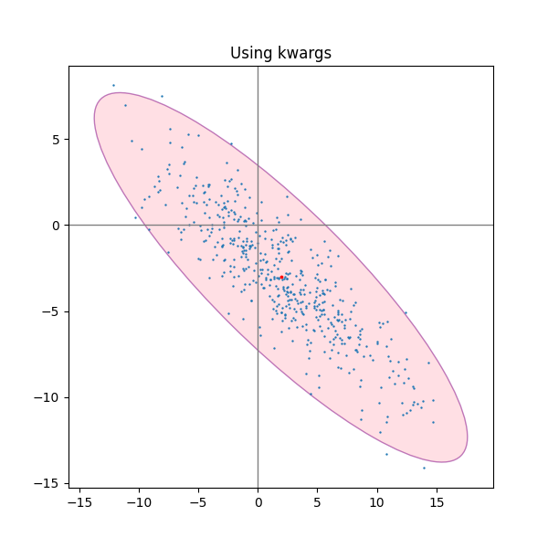
使用关键字参数

使用为指定的kwargsmatplotlib.patches.Patch以不同的方式渲染椭圆。

fig, ax_kwargs = plt.subplots(figsize=(6, 6))
dependency_kwargs = [[-0.8, 0.5],
                     [-0.2, 0.5]]
mu = 2, -3
scale = 6, 5

ax_kwargs.axvline(c='grey', lw=1)
ax_kwargs.axhline(c='grey', lw=1)

x, y = get_correlated_dataset(500, dependency_kwargs, mu, scale)
# Plot the ellipse with zorder=0 in order to demonstrate
# its transparency (caused by the use of alpha).
confidence_ellipse(x, y, ax_kwargs,
                   alpha=0.5, facecolor='pink', edgecolor='purple', zorder=0)

ax_kwargs.scatter(x, y, s=0.5)
ax_kwargs.scatter(mu[0], mu[1], c='red', s=3)
ax_kwargs.set_title('Using kwargs')

fig.subplots_adjust(hspace=0.25)
plt.show()