图像演示

在Matplotlib中绘制图像的许多方法。

在matplotlib中，最常见的绘制图像的方法是 imshow . 下面的示例演示了imshow的许多功能以及您可以创建的许多图像。

import numpy as np
import matplotlib.cm as cm
import matplotlib.pyplot as plt
import matplotlib.cbook as cbook
from matplotlib.path import Path
from matplotlib.patches import PathPatch


# Fixing random state for reproducibility
np.random.seed(19680801)

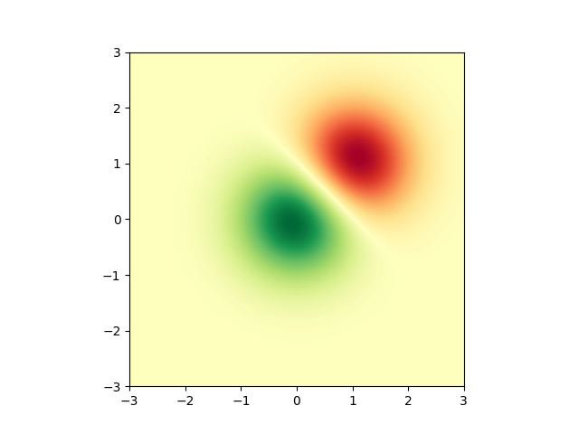
首先，我们将生成一个简单的二元正态分布。

delta = 0.025
x = y = np.arange(-3.0, 3.0, delta)
X, Y = np.meshgrid(x, y)
Z1 = np.exp(-X**2 - Y**2)
Z2 = np.exp(-(X - 1)**2 - (Y - 1)**2)
Z = (Z1 - Z2) * 2

fig, ax = plt.subplots()
im = ax.imshow(Z, interpolation='bilinear', cmap=cm.RdYlGn,
               origin='lower', extent=[-3, 3, -3, 3],
               vmax=abs(Z).max(), vmin=-abs(Z).max())

plt.show()

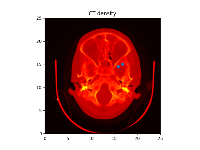
也可以显示图片的图像。

# A sample image
with cbook.get_sample_data('ada.png') as image_file:
    image = plt.imread(image_file)

fig, ax = plt.subplots()
ax.imshow(image)
ax.axis('off')  # clear x-axis and y-axis


# And another image

w, h = 512, 512

with cbook.get_sample_data('ct.raw.gz') as datafile:
    s = datafile.read()
A = np.frombuffer(s, np.uint16).astype(float).reshape((w, h))
A /= A.max()

fig, ax = plt.subplots()
extent = (0, 25, 0, 25)
im = ax.imshow(A, cmap=plt.cm.hot, origin='upper', extent=extent)

markers = [(15.9, 14.5), (16.8, 15)]
x, y = zip(*markers)
ax.plot(x, y, 'o')

ax.set_title('CT density')

plt.show()

• 
• 

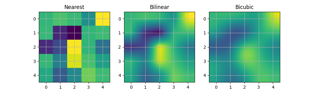
插值图像

也可以在显示图像之前插入图像。要小心，因为这可能会操纵数据的外观，但它有助于实现所需的外观。下面我们将显示相同的（小）数组，用三种不同的插值方法进行插值。

像素的中心 [i, j] 在（i+0.5，i+0.5）处绘制。如果使用interpolation='nearest'，以（i，j）和（i+1，j+1）为边界的区域将具有相同的颜色。如果使用插值，则像素中心将具有与“最近”相同的颜色，但其他像素将在相邻像素之间插值。

为了在执行插值时防止边缘效应，Matplotlib在输入数组的边缘周围填充相同的像素：如果您有一个5x5数组，颜色为a-y，如下所示：

a b c d e
f g h i j
k l m n o
p q r s t
u v w x y

Matplotlib计算填充数组上的插值和调整大小：

a a b c d e e
a a b c d e e
f f g h i j j
k k l m n o o
p p q r s t t
o u v w x y y
o u v w x y y

然后提取结果的中心区域。（Matplotlib的极旧版本（<0.63）没有填充数组，而是调整视图限制以隐藏受影响的边缘区域。）

这种方法允许在没有边缘效果的情况下绘制阵列的全部范围，例如，使用不同的插值方法将不同大小的多个图像叠放在另一个图像上—请参阅 图层图像 . 它还意味着性能下降，因为必须创建这个新的临时填充数组。复杂的插值也意味着性能下降；对于最大性能或非常大的图像，建议使用interpolation='nearest'。

A = np.random.rand(5, 5)

fig, axs = plt.subplots(1, 3, figsize=(10, 3))
for ax, interp in zip(axs, ['nearest', 'bilinear', 'bicubic']):
    ax.imshow(A, interpolation=interp)
    ax.set_title(interp.capitalize())
    ax.grid(True)

plt.show()

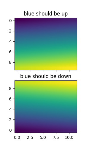
可以指定是否应使用数组原点X打印图像。 [0, 0] 在左上角或右下角使用原点参数。您还可以控制默认设置image.origin matplotlibrc file . 有关此主题的更多信息，请参阅 complete guide on origin and extent .

x = np.arange(120).reshape((10, 12))

interp = 'bilinear'
fig, axs = plt.subplots(nrows=2, sharex=True, figsize=(3, 5))
axs[0].set_title('blue should be up')
axs[0].imshow(x, origin='upper', interpolation=interp)

axs[1].set_title('blue should be down')
axs[1].imshow(x, origin='lower', interpolation=interp)
plt.show()

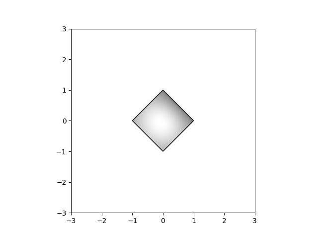
最后，我们将使用剪辑路径显示图像。

delta = 0.025
x = y = np.arange(-3.0, 3.0, delta)
X, Y = np.meshgrid(x, y)
Z1 = np.exp(-X**2 - Y**2)
Z2 = np.exp(-(X - 1)**2 - (Y - 1)**2)
Z = (Z1 - Z2) * 2

path = Path([[0, 1], [1, 0], [0, -1], [-1, 0], [0, 1]])
patch = PathPatch(path, facecolor='none')

fig, ax = plt.subplots()
ax.add_patch(patch)

im = ax.imshow(Z, interpolation='bilinear', cmap=cm.gray,
               origin='lower', extent=[-3, 3, -3, 3],
               clip_path=patch, clip_on=True)
im.set_clip_path(patch)

plt.show()

---

工具书类

本例中显示了以下函数和方法的使用：

import matplotlib
matplotlib.axes.Axes.imshow
matplotlib.pyplot.imshow
matplotlib.artist.Artist.set_clip_path
matplotlib.patches.PathPatch