阿贝尔沙堆模型
引言
这些注释介绍了Dhar的阿贝尔沙堆模型(ASM)和Sage沙堆,Sage沙堆是Sage中用于进行沙堆计算的工具集合。要更全面地介绍ASM理论,请参阅 Chip-Firing and Rotor-Routing on Directed Graphs [H] 由Holroyd等人撰写,以及 Riemann-Roch and Abel-Jacobi Theory on a Finite Graph 作者:Baker和Norine [BN] 是推荐的。另请参阅 [PPW2013].
为了描述ASM,我们从一个 sandpile graph :有向多重图 Gamma 使用顶点 s 从每个顶点都可以访问。通过 multigraph ,我们的意思是每一条边 Gamma 被分配一个非负整数权重。可以这么说 s 是 accessible 从某个顶点 v 表示存在从以下位置开始的有向边序列(可能为空 v 并在以下位置结束 s 。我们打电话给 s 这个 sink 尽管沙堆图形可能有向外的边,原因稍后将会清楚。
We denote the vertex set of Gamma by V, and define tilde{V} = Vsetminus{s}. For any vertex v, we let mbox{out-degree}(v) (the out-degree of v) be the sum of the weights of all edges leaving v.
构型和除数
A configuration on Gamma is an element of ZZ_{geq 0} tilde{V}, i.e., the assignment of a nonnegative integer to each nonsink vertex. We think of each integer as a number of grains of sand being placed at the corresponding vertex. A divisor on Gamma is an element of ZZ V, i.e., an element in the free abelian group on all of the vertices. In the context of divisors, it is sometimes useful to think of a divisor on Gamma as assigning dollars to each vertex, with negative integers signifying a debt.
稳定化
A configuration c is stable at a vertex vintilde{V} if c(v) < mbox{out-degree}(v). Otherwise, c is unstable at v. A configuration c (in itself) is stable if it is stable at each nonsink vertex. Otherwise, c is unstable. If c is unstable at v, the vertex v can be fired (toppled) by removing mbox{out-degree}(v) grains of sand from v and adding grains of sand to the neighbors of v, determined by the weights of the edges leaving v (each vertex w gets as many grains as the weight of the edge (v, w) is, if there is such an edge). Note that grains that are added to the sink s are not counted (i.e., they "disappear").
尽管我们的初衷是好的,但我们有时会考虑发射一个稳定的顶点,导致该顶点上的沙子数量为负值。我们也可能 reverse-fire 一个顶点,从顶点的邻居(包括水槽)吸收沙子。
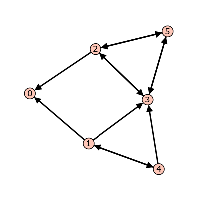
Example. 请看下面的图表:
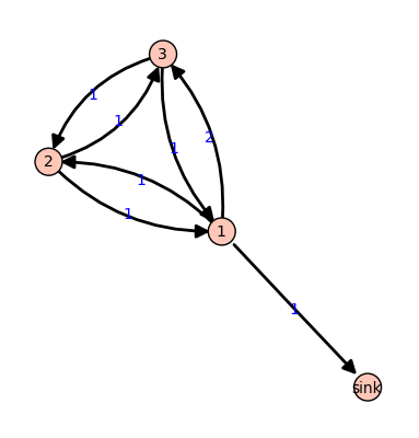
Gamma
所有边都具有权重 1 除了从顶点1到顶点3的边,它具有权重 2 。如果我们让 c = (5,0,1) 对于分别位于顶点1、2和3上的指定数量的沙粒,则只有出度为4的顶点1是不稳定的。发射顶点1提供了一个新的配置 c' = (1,1,3) 。这里, 4 颗粒离开了顶点1。其中一个已经到了下沉顶点(并且忘记了),一个已经到了顶点2,还有两个到了顶点3,因为从1到3的边具有权重 2 。新配置中的顶点3现在不稳定。此示例的Sage代码如下所示。**
sage: g = {0:{},
....:      1:{0:1, 2:1, 3:2},
....:      2:{1:1, 3:1},
....:      3:{1:1, 2:1}}
sage: S = Sandpile(g, 0)   # create the sandpile
sage: S.show(edge_labels=true)  # display the graph
创建配置::
sage: c = SandpileConfig(S, {1:5, 2:0, 3:1})
sage: S.out_degree()
{0: 0, 1: 4, 2: 2, 3: 2}
着火顶点 1 **
sage: c.fire_vertex(1)
{1: 1, 2: 1, 3: 3}
配置未更改::
sage: c
{1: 5, 2: 0, 3: 1}
重复发射顶点,直到配置变得稳定::
sage: c.stabilize()
{1: 2, 2: 1, 3: 1}
替代方案::
sage: ~c             # shorthand for c.stabilize()
{1: 2, 2: 1, 3: 1}
sage: c.stabilize(with_firing_vector=true)
[{1: 2, 2: 1, 3: 1}, {1: 2, 2: 2, 3: 3}]
由于顶点3在发射顶点1后变得不稳定,因此可以发射,这会导致顶点2变得不稳定,等等。重复发射最终会导致稳定的配置。上面的Sage代码的最后一行是一个列表,它的第一个元素是得到的稳定配置, (2,1,1) 。第二个分量记录每个顶点在稳定化过程中发射的次数。
由于接收器可以从每个非接收器顶点访问,并且从不触发,因此每个配置都将在有限数量的顶点触发后稳定下来。这并不明显,但所产生的稳定与不稳定顶点的激发顺序无关。因此,每种配置都稳定到唯一的稳定配置。
拉普拉斯
确定…的顶点的总顺序 Gamma ,从而导致通过数字对顶点进行标记 1, 2, ldots, n 对一些人来说 n (按给定顺序)。这个 Laplacian 的 Gamma 是
哪里 D 是顶点的出度的对角矩阵(即,对角线 n times n -矩阵,其 (i, i) -th条目是顶点的出度 i )和 A 是邻接矩阵,其 (i,j) -th条目是从顶点算起的边的权重 i 到顶点 j ,我们认为这是 0 如果没有优势的话。这个 reduced Laplacian , tilde{L} 是通过去除与汇点对应的行和列而形成的拉普拉斯矩阵的子矩阵。激发配置的顶点与减去约化的拉普拉斯量的相应行相同。
Example. (续)::
sage: S.vertices(sort=True)  # the ordering of the vertices
[0, 1, 2, 3]
sage: S.laplacian()
[ 0  0  0  0]
[-1  4 -1 -2]
[ 0 -1  2 -1]
[ 0 -1 -1  2]
sage: S.reduced_laplacian()
[ 4 -1 -2]
[-1  2 -1]
[-1 -1  2]
我们之前考虑的配置::
sage: c = SandpileConfig(S, [5,0,1])
sage: c
{1: 5, 2: 0, 3: 1}
激发顶点1等同于从配置中减去减少的拉普拉斯的对应行(视为向量):
sage: c.fire_vertex(1).values()
[1, 1, 3]
sage: S.reduced_laplacian()[0]
(4, -1, -2)
sage: vector([5,0,1]) - vector([4,-1,-2])
(1, 1, 3)
递归元素
想象一下,在一个实验中,沙粒一次一粒地落到图表上,然后暂停,让形状在两滴之间稳定下来。在此过程中,某些配置只能显示一次。例如,对于大多数图表,一旦将沙子放到图表上,添加沙子和稳定化的顺序都不会导致图表中没有沙子。其他配置-所谓的 recurrent configurations -当这个过程无限重复时,将无限频繁地出现。
准确地说,一种配置 c 是 recurrent 如果(I)它是稳定的,以及(Ii)给定任何配置 a ,有一种配置 b 以至于 c = mbox{stab}(a+b) ,稳定了 a + b 。
The maximal-stable configuration, denoted c_{mathrm{max}}, is defined by c_{mathrm{max}}(v)=mbox{out-degree}(v)-1 for all nonsink vertices v. It is clear that c_{mathrm{max}} is recurrent. Further, it is not hard to see that a configuration is recurrent if and only if it has the form mbox{stab}(a+c_{mathrm{max}}) for some configuration a.
Example. (续)::
sage: S.recurrents(verbose=false)
[[3, 1, 1], [2, 1, 1], [3, 1, 0]]
sage: c = SandpileConfig(S, [2,1,1])
sage: c
{1: 2, 2: 1, 3: 1}
sage: c.is_recurrent()
True
sage: S.max_stable()
{1: 3, 2: 1, 3: 1}
将任何配置添加到最大稳定配置并稳定会产生循环配置:
sage: x = SandpileConfig(S, [1,0,0])
sage: x + S.max_stable()
{1: 4, 2: 1, 3: 1}
使用 & 要添加和稳定:
sage: c = x & S.max_stable()
sage: c
{1: 3, 2: 1, 3: 0}
sage: c.is_recurrent()
True
请注意执行加法和稳定化的各种方法:
sage: m = S.max_stable()
sage: (x + m).stabilize() == ~(x + m)
True
sage: (x + m).stabilize() == x & m
True
烧录配置
A burning configuration is a ZZ_{geq 0}-linear combination f of the rows of the reduced Laplacian matrix having nonnegative entries and such that every vertex is accessible from some vertex in the support of f (in other words, for each vertex w, there is a path from some v in operatorname{supp} f to w). The corresponding burning script gives the coefficients in the ZZ_{geq 0}-linear combination needed to obtain the burning configuration. So if b is a burning configuration, sigma is its script, and tilde{L} is the reduced Laplacian, then sigma,tilde{L} = b. The minimal burning configuration is the one with the minimal script (each of its components is no larger than the corresponding component of any other script for a burning configuration).
在给定燃烧配置的情况下 b 有剧本 sigma ,以及任何配置 c 在同一张图上,以下内容是等价的:
c 是反复出现的;
c + b 稳定到 c ;
稳定化的激发矢量 c + b 是 sigma 。
燃烧配置和脚本是使用Speer的脚本算法的修改版本计算的。这是Dhar烧录算法的有向多图的推广。
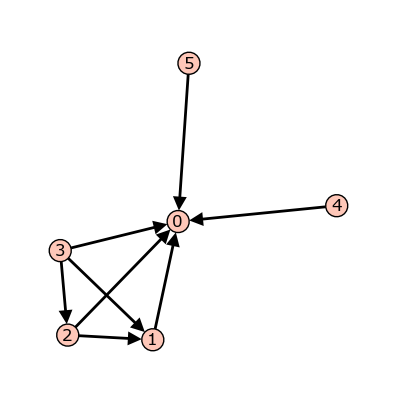
Example. **
sage: g = {0:{},1:{0:1,3:1,4:1},2:{0:1,3:1,5:1},
....:      3:{2:1,5:1},4:{1:1,3:1},5:{2:1,3:1}}
sage: G = Sandpile(g,0)
sage: G.burning_config()
{1: 2, 2: 0, 3: 1, 4: 1, 5: 0}
sage: G.burning_config().values()
[2, 0, 1, 1, 0]
sage: G.burning_script()
{1: 1, 2: 3, 3: 5, 4: 1, 5: 4}
sage: G.burning_script().values()
[1, 3, 5, 1, 4]
sage: matrix(G.burning_script().values())*G.reduced_laplacian()
[2 0 1 1 0]
沙堆群
稳定构型的集合形成了一个交换么半群,其加法定义为普通加法,然后是稳定化。身份元素是全零配置。当基础图是DAG(有向无环图)时,这个么半群就是群。
The recurrent elements form a submonoid which turns out to be a group. This group is called the sandpile group for Gamma, denoted mathcal{S}(Gamma). Its identity element is usually not the all-zero configuration (again, only in the case that Gamma is a DAG). So finding the identity element is an interesting problem.
Let n=|V|-1 and fix an ordering of the nonsink vertices. Let mathcal{tilde{L}}subsetZZ^n denote the column-span of tilde{L}^t, the transpose of the reduced Laplacian. It is a theorem that
因此,沙堆群的元素数为 det{tilde{L}} ,根据矩阵树定理,它是指向汇点的加权树的数量。
Example. (续)::
sage: S.group_order()
3
sage: S.invariant_factors()
[1, 1, 3]
sage: S.reduced_laplacian().dense_matrix().smith_form()
(
[1 0 0]  [ 1  0  0]  [1 3 5]
[0 1 0]  [ 0  1  0]  [1 4 6]
[0 0 3], [ 0 -1  1], [1 4 7]
)
将身份添加到任何循环配置并稳定会产生相同的循环配置:
sage: S.identity()
{1: 3, 2: 1, 3: 0}
sage: i = S.identity()
sage: m = S.max_stable()
sage: i & m == m
True
自组织临界性
沙堆模型是由Bak,Tang和Wiesenfeld在文中提出的, Self-organized criticality: an explanation of 1/ƒ noise [BTW]. 这一术语 self-organized criticality 没有精确的定义,但可以粗略地用来描述一个自然演变到几乎不稳定的状态的系统,这样不稳定就可以用幂定律来描述。在实践中, self-organized criticality 通常被认为是指 like the sandpile model on a grid graph 。栅格图只是一个带有额外汇点的栅格。每条边内部的折点都有一条通向水槽的边,角点有一条权重边 2 。因此,每个非下沉顶点都有出度。 4 。
想象一下,在一个空的栅格图上反复落下沙粒,让沙堆在中间稳定下来。起初几乎没有活动,但随着时间的推移,由一粒沙子引起的雪崩的大小和程度变得很难预测。计算机实验-我认为还没有证据-表明雪崩大小的分布服从指数为-1的幂定律。在下面的示例中,雪崩的大小被视为每个顶点发射次数的总和。
Example (distribution of avalanche sizes). **
sage: S = sandpiles.Grid(10,10)
sage: m = S.max_stable()
sage: a = []
sage: for i in range(10000):  # long time (15s on sage.math, 2012)
....:     m = m.add_random()
....:     m, f = m.stabilize(true)
....:     a.append(sum(f.values()))
...
sage: p = list_plot([[log(i+1),log(a.count(i))] for i in [0..max(a)] if a.count(i)])  # long time
sage: p.axes_labels(['log(N)','log(D(N))'])  # long time
sage: p  # long time
Graphics object consisting of 1 graphics primitive
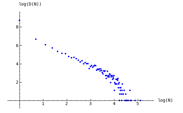
雪崩大小的分布
注意:在上面的代码中, m.stabilize(true) 返回由稳定配置和激发向量组成的列表。(省略 true 将只给出稳定的配置。)
因子与离散黎曼曲面
本节的参考文献为 Riemann-Roch and Abel-Jacobi theory on a finite graph [BN].
A divisor on Gamma is an element of the free abelian group on its vertices, including the sink. Suppose, as above, that the n+1 vertices of Gamma have been ordered, and that mathcal{L} is the column span of the transpose of the Laplacian. A divisor is then identified with an element DinZZ^{n+1}, and two divisors are linearly equivalent if they differ by an element of mathcal{L}. A divisor E is effective, written Egeq0, if E(v)geq0 for each vin V, i.e., if Einmathbb{Z}_{geq 0}^{n+1}. The degree of a divisor D is deg(D) := sum_{vin V} D(v). The divisors of degree zero modulo linear equivalence form the Picard group, or Jacobian of the graph. For an undirected graph, the Picard group is isomorphic to the sandpile group.
这个 complete linear system 对于除数 D ,表示为 |D| ,有效因子的集合是否线性地等价于 D 。
黎曼-罗赫
To describe the Riemann-Roch theorem in this context, suppose that Gamma is an undirected, unweighted graph. The dimension, r(D), of the linear system |D| is -1 if |D|=emptyset, and otherwise is the greatest integer s such that |D-E|neq0 for all effective divisors E of degree s. Define the canonical divisor by K = sum_{vin V} (deg(v)-2) v, and the genus by g = #(E) - #(V) + 1. The Riemann-Roch theorem says that for any divisor D,
Example. **
sage: G = sandpiles.Complete(5) # the sandpile on the complete graph with 5 vertices
图表上的除数::
sage: D = SandpileDivisor(G, [1,2,2,0,2])
验证Riemann-Roch定理:
sage: K = G.canonical_divisor()
sage: D.rank() - (K - D).rank() == D.deg() + 1 - G.genus()
True
与之线性等价的有效因子 D **
sage: D.effective_div(False)
[[0, 1, 1, 4, 1], [1, 2, 2, 0, 2], [4, 0, 0, 3, 0]]
达到线性等价的非特殊因子(次数因子 g-1 具有空线性系统):
sage: N = G.nonspecial_divisors()
sage: [E.values() for E in N[:5]]   # the first few
[[-1, 0, 1, 2, 3],
 [-1, 0, 1, 3, 2],
 [-1, 0, 2, 1, 3],
 [-1, 0, 2, 3, 1],
 [-1, 0, 3, 1, 2]]
sage: len(N)
24
sage: len(N) == G.h_vector()[-1]
True
描绘线性系统
确定除数 D 。至少有两个自然图与线性系统相关联 D 。首先,考虑具有顶点集的有向图 |D| 并且从顶点开始有一条边 E 到顶点 F 如果 F 是通过以下方式获得的 E 通过发射单个不稳定的顶点。**
sage: S = Sandpile(graphs.CycleGraph(6),0)
sage: D = SandpileDivisor(S, [1,1,1,1,2,0])
sage: D.is_alive()
True
sage: eff = D.effective_div()
sage: firing_graph(S,eff).show3d(edge_size=.005,vertex_size=0.01,iterations=500)
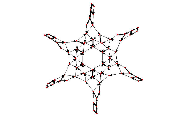
系统的完全线性系统 (1,1,1,1,2,0) 在……上面 C_6 :单发射击
这个 is_alive 方法检查除数是否为 D 是活的,即每个除数是否线性等于 D 是不稳定的。
第二个图具有相同的顶点集,但有一条边来自 E 至 F 如果 F 从以下来源获得 E 通过激发所有不稳定的顶点 E 。**
sage: S = Sandpile(graphs.CycleGraph(6),0)
sage: D = SandpileDivisor(S, [1,1,1,1,2,0])
sage: eff = D.effective_div()
sage: parallel_firing_graph(S,eff).show3d(edge_size=.005,vertex_size=0.01,iterations=500)
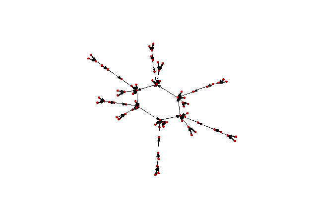
系统的完全线性系统 (1,1,1,1,2,0) 在……上面 C_6 :并行发射
请注意,在上面的每个示例中,从线性系统中的任何除数开始并跟随边,最终将一个人引入一个长度循环 6 (循环使用除数 (1,1,1,1,2,0) )。因此, D.alive() 退货 True 。在Sage中,人们可以旋转上面的图形来更好地了解结构。
沙堆的代数几何
仿射
Let n = |V| - 1, and fix an ordering on the nonsink vertices of Gamma. Let tilde{mathcal{L}} subset ZZ^n denote the column-span of tilde{L}^t, the transpose of the reduced Laplacian. Label vertex i with the indeterminate x_i, and let CC[Gamma_s] = CC[x_1, dots, x_n]. (Here, s denotes the sink vertex of Gamma.) The sandpile ideal or toppling ideal, first studied by Cori, Rossin, and Salvy [CRS] for undirected graphs, is the lattice ideal for tilde{mathcal{L}}:
哪里 x^u := prod_{i=1}^n x^{u_i} 为 u in ZZ^n 。
For each cinZZ^n define t(c) = x^{c^+} - x^{c^-} where c^+_i = max{c_i,0} and c^-_i = max{-c_i,0}, so that c = c^+ - c^-. Then, for each sigma in ZZ^n, define T(sigma) = t(tilde{L}^tsigma). It then turns out that
哪里 e_i 是 i -第th标准基向量和 b 是任何烧录配置。
The affine coordinate ring, CC[Gamma_s]/I, is isomorphic to the group algebra of the sandpile group, CC[mathcal{S}(Gamma)].
标准术语--排序 CC[Gamma_s] 与词典编排顺序相反 x_i > x_j 如果顶点 v_i 与折点相比,距离汇点更远 v_j 。(对于与水槽等距离的顶点,可以进行选择。)如果 sigma_b 是刻录配置的脚本(不一定是最低配置),那么
是Gröbner的基础 I 。
射影
Now let CC[Gamma] = CC[x_0,x_1,dots,x_n], where x_0 corresponds to the sink vertex. The homogeneous sandpile ideal, denoted I^h, is obtaining by homogenizing I with respect to x_0. Let L be the (full) Laplacian, and mathcal{L} subset ZZ^{n+1} be the column span of its transpose, L^t. Then I^h is the lattice ideal for mathcal{L}:
这个理想可以通过使理想饱和来计算。
关于不定数的乘积: prod_{i=0}^n x_i (延长 T 运算符)。关于上述程度词典顺序的Gröbner基(具有 x_0 最小顶点)是通过使非均匀沙堆理想的Gröbner基的每个元素关于 x_0 。
Example. **
sage: g = {0:{},1:{0:1,3:1,4:1},2:{0:1,3:1,5:1},
....:      3:{2:1,5:1},4:{1:1,3:1},5:{2:1,3:1}}
sage: S = Sandpile(g, 0)
sage: S.ring()
Multivariate Polynomial Ring in x5, x4, x3, x2, x1, x0 over Rational Field
理想的均匀沙堆::
sage: S.ideal()
Ideal (x2 - x0, x3^2 - x5*x0, x5*x3 - x0^2, x4^2 - x3*x1, x5^2 - x3*x0,
x1^3 - x4*x3*x0, x4*x1^2 - x5*x0^2) of Multivariate Polynomial Ring
in x5, x4, x3, x2, x1, x0 over Rational Field
理想的创造者::
sage: S.ideal(true)
[x2 - x0,
 x3^2 - x5*x0,
 x5*x3 - x0^2,
 x4^2 - x3*x1,
 x5^2 - x3*x0,
 x1^3 - x4*x3*x0,
 x4*x1^2 - x5*x0^2]
其决议::
sage: S.resolution() # long time
'R^1 <-- R^7 <-- R^19 <-- R^25 <-- R^16 <-- R^4'
和Betti桌子::
sage: S.betti() # long time
           0     1     2     3     4     5
------------------------------------------
    0:     1     1     -     -     -     -
    1:     -     4     6     2     -     -
    2:     -     2     7     7     2     -
    3:     -     -     6    16    14     4
------------------------------------------
total:     1     7    19    25    16     4
希尔伯特函数::
sage: S.hilbert_function()
[1, 5, 11, 15]
以及它的第一个差异(计算每个度数的超稳构型数):
sage: S.h_vector()
[1, 4, 6, 4]
sage: x = [i.deg() for i in S.superstables()]
sage: sorted(x)
[0, 1, 1, 1, 1, 2, 2, 2, 2, 2, 2, 3, 3, 3, 3]
希尔伯特函数开始等于希尔伯特多项式的次数,后者在沙堆理想的情况下始终是一个常数:
sage: S.postulation()
3
零
这个 zero set 对于沙堆的理想 I 是
the set of simultaneous zeros of the polynomials in I. Letting S^1 denote the unit circle in the complex plane, Z(I) is a finite subgroup of S^1 times cdots times S^1 subset CC^n, isomorphic to the sandpile group. The zero set is actually linearly isomorphic to a faithful representation of the sandpile group on CC^n.
Example. (续)::
sage: S = Sandpile({0: {}, 1: {2: 2}, 2: {0: 4, 1: 1}}, 0)
sage: S.ideal().gens()
[x1^2 - x2^2, x1*x2^3 - x0^4, x2^5 - x1*x0^4]
接近零点设置(设置 x_0 = 1 ):
sage: S.solve()
[[-0.707107000000000 + 0.707107000000000*I,
  0.707107000000000 - 0.707107000000000*I],
 [-0.707107000000000 - 0.707107000000000*I,
  0.707107000000000 + 0.707107000000000*I],
 [-I, -I],
 [I, I],
 [0.707107000000000 + 0.707107000000000*I,
  -0.707107000000000 - 0.707107000000000*I],
 [0.707107000000000 - 0.707107000000000*I,
  -0.707107000000000 + 0.707107000000000*I],
 [1, 1],
 [-1, -1]]
sage: len(_) == S.group_order()
True
这些零由单个向量作为一组生成::
sage: S.points()
[[-(1/2*I + 1/2)*sqrt(2), (1/2*I + 1/2)*sqrt(2)]]
决议
The homogeneous sandpile ideal, I^h, has a free resolution graded by the divisors on Gamma modulo linear equivalence. (See the section on Discrete Riemann Surfaces for the language of divisors and linear equivalence.) Let S = CC[Gamma] = CC[x_0,dots,x_n], as above, and let mathfrak{S} denote the group of divisors modulo rational equivalence. Then S is graded by mathfrak{S} by letting deg(x^c) = c in mathfrak{S} for each monomial x^c. The minimal free resolution of I^h has the form
凡. beta_{i,D} 是 Betti numbers 为 I^h 。
对于每个除数类 Dinmathfrak{S} ,定义了单纯复形
Betti数 beta_{i,D} 等于尺寸超过 CC 的 i -TH约化同调群 Delta_D :
sage: S = Sandpile({0:{},1:{0: 1, 2: 1, 3: 4},2:{3: 5},3:{1: 1, 2: 1}},0)
具有非平凡同调的所有除数类的代表::
sage: p = S.betti_complexes()
sage: p[0]
[{0: -8, 1: 5, 2: 4, 3: 1},
 Simplicial complex with vertex set (1, 2, 3) and facets {(3,), (1, 2)}]
与列表中第一个除数相关联的同调::
sage: D = p[0][0]
sage: D.effective_div()
[{0: 0, 1: 0, 2: 0, 3: 2}, {0: 0, 1: 1, 2: 1, 3: 0}]
sage: [E.support() for E in D.effective_div()]
[[3], [1, 2]]
sage: D.Dcomplex()
Simplicial complex with vertex set (1, 2, 3) and facets {(3,), (1, 2)}
sage: D.Dcomplex().homology()
{0: Z, 1: 0}
最小自由分辨率::
sage: S.resolution()
'R^1 <-- R^5 <-- R^5 <-- R^1'
sage: S.betti()
           0     1     2     3
------------------------------
    0:     1     -     -     -
    1:     -     5     5     -
    2:     -     -     -     1
------------------------------
total:     1     5     5     1
sage: len(p)
11
表中每个元素的同调群的度和秩数 p (对比上图中的Betti表):
sage: [[sum(d[0].values()),d[1].betti()] for d in p]
[[2, {0: 2, 1: 0}],
 [3, {0: 1, 1: 1, 2: 0}],
 [2, {0: 2, 1: 0}],
 [3, {0: 1, 1: 1, 2: 0}],
 [2, {0: 2, 1: 0}],
 [3, {0: 1, 1: 1, 2: 0}],
 [2, {0: 2, 1: 0}],
 [3, {0: 1, 1: 1}],
 [2, {0: 2, 1: 0}],
 [3, {0: 1, 1: 1, 2: 0}],
 [5, {0: 1, 1: 0, 2: 1}]]
完全交与算术Gorenstein颠覆理想
注意:在上一节中,请注意解析的长度始终为 n 既然理想是科恩-麦考利。
去做。
无向图的Betti数
去做。
用法
初始化
Sage中的沙堆结构主要有三类: Sandpile , SandpileConfig ,以及 SandpileDivisor 。初始化 Sandpile 具有以下形式::
.. skip
Sage:S=沙堆(图形,下沉)
哪里 graph 表示一个图形,并且 sink 是水槽顶点的关键点。有四种可能的形式 graph :
一本Python词典::
sage: g = {0: {}, 1: {0: 1, 3: 1, 4: 1}, 2: {0: 1, 3: 1, 5: 1},
....:      3: {2: 1, 5: 1}, 4: {1: 1, 3: 1}, 5: {2: 1, 3: 1}}
词典中的图表。
每个关键点都是顶点的名称。每个顶点名称旁边 v 是一本由配对组成的词典:
vertex: weight。每一对都表示从 v 并在以下位置结束vertex具有等于(非负整数)权重的weight。允许循环。在上面的示例中,所有权重都是1。一个Python列表词典::
sage: g = {0: [], 1: [0, 3, 4], 2: [0, 3, 5],
....:      3: [2, 5], 4: [1, 3], 5: [2, 3]}
这是所有边权重等于1时的速记。上面的示例是针对相同显示的图形的。
Sage图(类型)
sage.graphs.graph.Graph):sage: g = graphs.CycleGraph(5) sage: S = Sandpile(g, 0) sage: type(g) <class 'sage.graphs.graph.Graph'>
要查看内置图形的类型,请输入
graphs.,包括期间,并按TAB键。Sage有向图::
sage: S = Sandpile(digraphs.RandomDirectedGNC(6), 0)
sage: S.show()
一张随机图。
看见 sage.graphs.graph_generators 有关Sage图形库和图形构造函数的更多信息。
这四种格式中的每一种都由沙堆类进行预处理,因此在内部,图形由最初呈现的字典字典格式表示。此内部格式由返回 dict() **
sage: S = Sandpile({0:[], 1:[0, 3, 4], 2:[0, 3, 5], 3: [2, 5], 4: [1, 3], 5: [2, 3]},0)
sage: S.dict()
{0: {},
 1: {0: 1, 3: 1, 4: 1},
 2: {0: 1, 3: 1, 5: 1},
 3: {2: 1, 5: 1},
 4: {1: 1, 3: 1},
 5: {2: 1, 3: 1}}
备注
用户负责确保每个顶点具有到指定接收器的有向路径。如果水槽有外边,则在沙堆计算时将忽略这些边(但不会对除数进行计算)。
用于检查给定顶点是否为接收器的代码::
sage: S = Sandpile({0:[], 1:[0, 3, 4], 2:[0, 3, 5], 3: [2, 5], 4: [1, 3], 5: [2, 3]},0)
sage: [S.distance(v,0) for v in S.vertices(sort=True)] # 0 is a sink
[0, 1, 1, 2, 2, 2]
sage: [S.distance(v,1) for v in S.vertices(sort=True)] # 1 is not a sink
[+Infinity, 0, +Infinity, +Infinity, 1, +Infinity]
方法
以下是以下摘要 Sandpile , SandpileConfig ,以及 SandpileDivisor 方法(函数)。每个摘要后面都有一个方法的完整描述列表。有更多的方法可用于沙堆,例如,从类DiGraph继承的方法。要查看全部内容,请输入 dir(Sandpile) 或键入 Sandpile. ,包括期间,并按TAB键。
沙堆
Summary of methods.
all_k_config -所有值都设置为k的常量配置。
all_k_div -所有值都设置为k的除数。
avalanche_polynomial -雪崩多项式。
betti -均匀倾覆理想的Betti表。
betti_complexes -具有非平凡同调的支持络合物。
burning_config -最小烧录配置。
burning_script -用于最低刻录配置的脚本。
canonical_divisor -标准除数。
dict -代表有向图的词典的词典。
genus -亏格:(#非循环边)-(#顶点)+1。
groebner -齐次倾覆理想的Groebner基。
group_gens -沙堆组的最小生成器列表。
group_order -沙堆群的大小。
h_vector -每个度数的超稳构型数。
help -特定于沙堆的方法列表(非继承自Graph)。
hilbert_function -齐次倾倒理想的希尔伯特函数。
ideal -饱和均匀倾覆理想。
identity -身份配置。
in_degree -顶点的入度或所有入度的列表。
invariant_factors -沙堆群的不变因子。
is_undirected -底层图形是否是无向的?
jacobian_representatives -雅可比群元素的代表。
laplacian -图的拉普拉斯矩阵。
markov_chain -配置或因子的沙堆马尔可夫链。
max_stable -最大稳定构型。
max_stable_div -最大稳定因子。
max_superstables -最大超稳构型。
min_recurrents -最小回归元。
nonsink_vertices -非沉点顶点。
nonspecial_divisors -非特殊因子。
out_degree --- The out-degree of a vertex or a list of all out-degrees.
picard_representatives -Picard群中d次除数类的表示。
points -沙堆理想的零点乘法群的生成元。
postulation -颠覆理想的假设数。
recurrents -循环构型。
reduced_laplacian -图的约化拉普拉斯矩阵。
reorder_vertices -颠倒了顶点名称的沙堆副本。
resolution -齐次倾覆理想的最小自由分解。
ring -包含均匀倾覆理想的环。
show -画出下面的图表。
show3d -画出下面的图表。
sink -下沉顶点。
smith_form -拉普拉斯函数的Smith范式。
solve -沙堆理想的复仿射零点的近似。
stable_configs -所有稳定配置的生成器。
stationary_density -沙堆的固定密度。
superstables -超稳构型。
symmetric_recurrents -对称递归构型。
tutte_polynomial -图特多项式。
unsaturated_ideal -不饱和的同质颠覆理想。
version -Sage沙堆的版本号。
zero_config -全零配置。
zero_div -全零除数。
Complete descriptions of Sandpile methods.
--
all_k_config(k)
将所有值设置为的常量配置 k 。
输入:
k --整型
输出:
SandpileConfig
示例:
sage: s = sandpiles.Diamond()
sage: s.all_k_config(7)
{1: 7, 2: 7, 3: 7}
--
all_k_div(k)
所有值都设置为的除数 k 。
输入:
k --整型
输出:
SandpileDivisor
示例:
sage: S = sandpiles.House()
sage: S.all_k_div(7)
{0: 7, 1: 7, 2: 7, 3: 7, 4: 7}
--
avalanche_polynomial(multivariable=True)
雪崩多项式。有关详细信息,请参阅备注。
输入:
multivariable --(默认: True )布尔型
输出:
多项式
示例:
sage: s = sandpiles.Complete(4)
sage: s.avalanche_polynomial()
9*x0*x1*x2 + 2*x0*x1 + 2*x0*x2 + 2*x1*x2 + 3*x0 + 3*x1 + 3*x2 + 24
sage: s.avalanche_polynomial(False)
9*x0^3 + 6*x0^2 + 9*x0 + 24
备注
对于每个非沉点顶点 v ,让 x_v 成为一个不确定的人。如果 (r,v) 是由常返数组成的对 r 和非沉点顶点 v ,则对于每个非沉点顶点 w ,让 n_w 是顶点的次数 w 火势在稳定中 r + v 。让我们 M(r,v) 做单项 prod_w x_w^{n_w} 也就是说,指数记录了 n_w AS w 在非沉没顶点上的范围。那么雪崩多项式就是 M(r,v) AS r 经常性租金的范围和 v 在非沉没顶点上的范围。如果 multivariable 是 False ,然后将所有不确定数设置为彼此相等(因此,只计算稳定化中的顶点激发次数,而忘记激发了哪些特定顶点)。
--
betti(verbose=True)
均匀倾覆理想的Betti表。如果 verbose 是 True ,它将打印标准的Betti表,否则,它将返回一个格式较差的表。
输入:
verbose --(默认: True )布尔型
输出:
沙堆的Betti数
示例:
sage: S = sandpiles.Diamond()
sage: S.betti()
           0     1     2     3
------------------------------
    0:     1     -     -     -
    1:     -     2     -     -
    2:     -     4     9     4
------------------------------
total:     1     6     9     4
sage: S.betti(False)
[1, 6, 9, 4]
--
betti_complexes()
具有非平凡同调的支撑络合物。(请参阅备注。)
输出:
(配对列表) [divisors, corresponding simplicial complex] )
示例:
sage: S = Sandpile({0:{},1:{0: 1, 2: 1, 3: 4},2:{3: 5},3:{1: 1, 2: 1}},0)
sage: p = S.betti_complexes()
sage: p[0]
[{0: -8, 1: 5, 2: 4, 3: 1}, Simplicial complex with vertex set (1, 2, 3) and facets {(3,), (1, 2)}]
sage: S.resolution()
'R^1 <-- R^5 <-- R^5 <-- R^1'
sage: S.betti()
           0     1     2     3
------------------------------
    0:     1     -     -     -
    1:     -     5     5     -
    2:     -     -     -     1
------------------------------
total:     1     5     5     1
sage: len(p)
11
sage: p[0][1].homology()
{0: Z, 1: 0}
sage: p[-1][1].homology()
{0: 0, 1: 0, 2: Z}
备注
A support-complex 是由线性系统中的约数的支点构成的单纯复形。
--
burning_config()
最小烧录配置。
输出:
DICT(配置)
示例:
sage: g = {0:{},1:{0:1,3:1,4:1},2:{0:1,3:1,5:1}, \
           3:{2:1,5:1},4:{1:1,3:1},5:{2:1,3:1}}
sage: S = Sandpile(g,0)
sage: S.burning_config()
{1: 2, 2: 0, 3: 1, 4: 1, 5: 0}
sage: S.burning_config().values()
[2, 0, 1, 1, 0]
sage: S.burning_script()
{1: 1, 2: 3, 3: 5, 4: 1, 5: 4}
sage: script = S.burning_script().values()
sage: script
[1, 3, 5, 1, 4]
sage: matrix(script)*S.reduced_laplacian()
[2 0 1 1 0]
备注
燃烧配置和脚本是使用Speer的脚本算法的修改版本计算的。这是Dhar烧录算法的有向多图的推广。
A burning configuration is a nonnegative integer-linear combination of the rows of the reduced Laplacian matrix having nonnegative entries and such that every vertex has a path from some vertex in its support. The corresponding burning script gives the integer-linear combination needed to obtain the burning configuration. So if b is the burning configuration, sigma is its script, and tilde{L} is the reduced Laplacian, then sigmacdot tilde{L} = b. The minimal burning configuration is the one with the minimal script (its components are no larger than the components of any other script for a burning configuration).
以下内容等同于配置 c 具有刻录配置 b 有剧本 sigma :
c 是反复出现的;
c+b 稳定到 c ;
稳定化的激发矢量 c+b 是 sigma 。
--
burning_script()
用于最小刻录配置的脚本。
输出:
迪克特
示例:
sage: g = {0:{},1:{0:1,3:1,4:1},2:{0:1,3:1,5:1},\
3:{2:1,5:1},4:{1:1,3:1},5:{2:1,3:1}}
sage: S = Sandpile(g,0)
sage: S.burning_config()
{1: 2, 2: 0, 3: 1, 4: 1, 5: 0}
sage: S.burning_config().values()
[2, 0, 1, 1, 0]
sage: S.burning_script()
{1: 1, 2: 3, 3: 5, 4: 1, 5: 4}
sage: script = S.burning_script().values()
sage: script
[1, 3, 5, 1, 4]
sage: matrix(script)*S.reduced_laplacian()
[2 0 1 1 0]
备注
燃烧配置和脚本是使用Speer的脚本算法的修改版本计算的。这是Dhar烧录算法的有向多图的推广。
A burning configuration 是具有非负条目的约化拉普拉斯矩阵的行的非负整数-线性组合,并且使得每个顶点都有从其支撑点的某个顶点的路径。相应的 burning script 给出了获得燃烧配置所需的整数线性组合。所以如果 b 是燃烧配置, s 是它的剧本,而且 L_{mathrm{red}} 是约化的拉普拉斯,那么 scdot L_{mathrm{red}}= b 。这个 minimal burning configuration 是具有最小脚本的脚本(其组件不大于烧录配置的任何其他脚本的组件)。
以下内容等同于配置 c 具有刻录配置 b 有剧本 s :
c 是反复出现的;
c+b 稳定到 c ;
稳定化的激发矢量 c+b 是 s 。
--
canonical_divisor()
正则除数。这是除数和 deg(v)-2 每个顶点上的沙粒(不包括循环)。仅适用于无向图。
输出:
SandpileDivisor
示例:
sage: S = sandpiles.Complete(4)
sage: S.canonical_divisor()
{0: 1, 1: 1, 2: 1, 3: 1}
sage: s = Sandpile({0:[1,1],1:[0,0,1,1,1]},0)
sage: s.canonical_divisor()  # loops are disregarded
{0: 0, 1: 0}
警告
底层图形必须是无方向的。
--
dict()
表示有向图的词典的词典。
输出:
迪克特
示例:
sage: S = sandpiles.Diamond()
sage: S.dict()
{0: {1: 1, 2: 1},
 1: {0: 1, 2: 1, 3: 1},
 2: {0: 1, 1: 1, 3: 1},
 3: {1: 1, 2: 1}}
sage: S.sink()
0
--
genus()
亏格:(#非循环边)-(#顶点)+1。仅定义为无向图。
输出:
整数
示例:
sage: sandpiles.Complete(4).genus()
3
sage: sandpiles.Cycle(5).genus()
1
--
groebner()
齐次倾覆理想的一个Groebner基。它是根据标准沙堆排序进行计算的(请参见 ring )。
输出:
Groebner基
示例:
sage: S = sandpiles.Diamond()
sage: S.groebner()
[x3*x2^2 - x1^2*x0, x2^3 - x3*x1*x0, x3*x1^2 - x2^2*x0, x1^3 - x3*x2*x0, x3^2 - x0^2, x2*x1 - x0^2]
--
group_gens(verbose=True)
沙堆组的最小生成器列表。如果 verbose 是 False 然后,生成器被表示为整数列表。
输入:
verbose --(默认: True )布尔型
输出:
沙堆配置列表(或整数列表,如果 verbose 是 False )
示例:
sage: s = sandpiles.Cycle(5)
sage: s.group_gens()
[{1: 0, 2: 1, 3: 1, 4: 1}]
sage: s.group_gens()[0].order()
5
sage: s = sandpiles.Complete(5)
sage: s.group_gens(False)
[[2, 3, 2, 2], [2, 2, 3, 2], [2, 2, 2, 3]]
sage: [i.order() for i in s.group_gens()]
[5, 5, 5]
sage: s.invariant_factors()
[1, 5, 5, 5]
--
group_order()
沙堆群的大小。
输出:
整数
示例:
sage: S = sandpiles.House()
sage: S.group_order()
11
--
h_vector()
每个度数中的超稳定构型数。等价地,这是(齐次)颠覆理想的希尔伯特函数的第一差分表。
输出:
非负整数列表
示例:
sage: s = sandpiles.Grid(2,2)
sage: s.hilbert_function()
[1, 5, 15, 35, 66, 106, 146, 178, 192]
sage: s.h_vector()
[1, 4, 10, 20, 31, 40, 40, 32, 14]
--
help(verbose=True)
沙堆特定方法的列表(不是从Graph继承的)。如果 verbose ,包括简短的描述。
输入:
verbose --(默认: True )布尔型
输出:
打印字符串
示例:
sage: Sandpile.help()
For detailed help with any method FOO listed below,
enter "Sandpile.FOO?" or enter "S.FOO?" for any Sandpile S.
<BLANKLINE>
all_k_config             -- The constant configuration with all values set to k.
all_k_div                -- The divisor with all values set to k.
avalanche_polynomial     -- The avalanche polynomial.
betti                    -- The Betti table for the homogeneous toppling ideal.
betti_complexes          -- The support-complexes with non-trivial homology.
...
unsaturated_ideal        -- The unsaturated, homogeneous toppling ideal.
version                  -- The version number of Sage Sandpiles.
zero_config              -- The all-zero configuration.
zero_div                 -- The all-zero divisor.
--
hilbert_function()
齐次倾覆理想的希尔伯特函数。
输出:
非负整数列表
示例:
sage: s = sandpiles.Wheel(5)
sage: s.hilbert_function()
[1, 5, 15, 31, 45]
sage: s.h_vector()
[1, 4, 10, 16, 14]
--
ideal(gens=False)
饱和均匀倾覆理想。如果 gens 是 True 作为替代,理想的发电机将被退还。
输入:
gens --(默认: False )布尔型
输出:
理想,或者可选的,理想的生成器
示例:
sage: S = sandpiles.Diamond()
sage: S.ideal()
Ideal (x2*x1 - x0^2, x3^2 - x0^2, x1^3 - x3*x2*x0, x3*x1^2 - x2^2*x0, x2^3 - x3*x1*x0, x3*x2^2 - x1^2*x0) of Multivariate Polynomial Ring in x3, x2, x1, x0 over Rational Field
sage: S.ideal(True)
[x2*x1 - x0^2, x3^2 - x0^2, x1^3 - x3*x2*x0, x3*x1^2 - x2^2*x0, x2^3 - x3*x1*x0, x3*x2^2 - x1^2*x0]
sage: S.ideal().gens()  # another way to get the generators
[x2*x1 - x0^2, x3^2 - x0^2, x1^3 - x3*x2*x0, x3*x1^2 - x2^2*x0, x2^3 - x3*x1*x0, x3*x2^2 - x1^2*x0]
--
identity(verbose=True)
身份配置。如果 verbose 是 False ,则将配置转换为整数列表。
输入:
verbose --(默认: True )布尔型
输出:
SandpileConfig或整数列表(如果为 verbose 是 False ,则将配置转换为整数列表。
示例:
sage: s = sandpiles.Diamond()
sage: s.identity()
{1: 2, 2: 2, 3: 0}
sage: s.identity(False)
[2, 2, 0]
sage: s.identity() & s.max_stable() == s.max_stable()
True
--
in_degree(v=None)
顶点的入度或所有入度的列表。
输入:
v --(可选)顶点名称
输出:
整数或DICT
示例:
sage: s = sandpiles.House()
sage: s.in_degree()
{0: 2, 1: 2, 2: 3, 3: 3, 4: 2}
sage: s.in_degree(2)
3
--
invariant_factors()
砂堆群的不变因子。
输出:
整数列表
示例:
sage: s = sandpiles.Grid(2,2)
sage: s.invariant_factors()
[1, 1, 8, 24]
--
is_undirected()
底层图形是否是无向的? True 如果 (u,v) 为AND EDGE当且仅当 (v,u) 是一条边,每条边都有相同的权重。
输出:
布尔型
示例:
sage: sandpiles.Complete(4).is_undirected()
True
sage: s = Sandpile({0:[1,2], 1:[0,2], 2:[0]}, 0)
sage: s.is_undirected()
False
--
jacobian_representatives(verbose=True)
雅各比集团成员的代表。如果 verbose 是 False ,则返回表示除数的列表。
输入:
verbose --(默认: True )布尔型
输出:
沙堆除数列表(或表示除数的列表)
示例:
对于无向图,形式的因子 s - deg(s)*sink AS s 不同的超级稳定器形成了一组不同的雅各布派代表。
sage: s = sandpiles.Complete(3)
sage: s.superstables(False)
[[0, 0], [0, 1], [1, 0]]
sage: s.jacobian_representatives(False)
[[0, 0, 0], [-1, 0, 1], [-1, 1, 0]]
如果该图是有向的,则上述表示可以通过等价地模拉普拉斯矩阵的行跨度:
sage: s = Sandpile({0: {1: 1, 2: 2}, 1: {0: 2, 2: 4}, 2: {0: 4, 1: 2}},0)
sage: s.group_order()
28
sage: s.jacobian_representatives()
[{0: -5, 1: 3, 2: 2}, {0: -4, 1: 3, 2: 1}]
让我们 tau 作为拉普拉斯算子转置的核的非负生成元,并令 tau_s 如果它是下沉分量,则沙堆群同构于阶循环群的直和 tau_s 以及雅各比集团。在上面的示例中,我们有:
sage: s.laplacian().left_kernel()
Free module of degree 3 and rank 1 over Integer Ring
Echelon basis matrix:
[14  5  8]
备注
雅可比群是以拉普拉斯矩阵的整数行跨度为模的所有零次除数的集合。
--
laplacian()
图的拉普拉斯矩阵。它的 rows 对顶点激发规则进行编码。
输出:
矩阵
示例:
sage: G = sandpiles.Diamond()
sage: G.laplacian()
[ 2 -1 -1  0]
[-1  3 -1 -1]
[-1 -1  3 -1]
[ 0 -1 -1  2]
警告
该功能 laplacian_matrix 应该避免。它返回拉普拉斯的索引版本。
--
markov_chain(state, distrib=None)
配置或因子的沙堆马尔可夫链。连锁店的起始点是 state 。有关详细信息,请参阅备注。
输入:
state--表示其中之一的SandpileConfig、SandpileDivisor或Listdistrib--(可选)非负数列表,总和为1(表示问题。Dist.)
输出:
马尔可夫链的生成器(见注)
示例:
sage: s = sandpiles.Complete(4)
sage: m = s.markov_chain([0,0,0])
sage: next(m)          # random
{1: 0, 2: 0, 3: 0}
sage: next(m).values() # random
[0, 0, 0]
sage: next(m).values() # random
[0, 0, 0]
sage: next(m).values() # random
[0, 0, 0]
sage: next(m).values() # random
[0, 1, 0]
sage: next(m).values() # random
[0, 2, 0]
sage: next(m).values() # random
[0, 2, 1]
sage: next(m).values() # random
[1, 2, 1]
sage: next(m).values() # random
[2, 2, 1]
sage: m = s.markov_chain(s.zero_div(), [0.1,0.1,0.1,0.7])
sage: next(m).values() # random
[0, 0, 0, 1]
sage: next(m).values() # random
[0, 0, 1, 1]
sage: next(m).values() # random
[0, 0, 1, 2]
sage: next(m).values() # random
[1, 1, 2, 0]
sage: next(m).values() # random
[1, 1, 2, 1]
sage: next(m).values() # random
[1, 1, 2, 2]
sage: next(m).values() # random
[1, 1, 2, 3]
sage: next(m).values() # random
[1, 1, 2, 4]
sage: next(m).values() # random
[1, 1, 3, 4]
备注
这个 closed sandpile Markov chain 具有由沙堆上的配置组成的状态空间。它通过随机选择顶点(根据概率分布)从一个状态转换 distrib ),在该顶点处撒下一粒沙子,然后稳定下来。如果选定的顶点是水槽,链将保持当前状态。
这个 open sandpile Markov chain 具有由递归元素组成的状态空间,即状态空间为沙堆群。它从配置过渡到 c 通过选择顶点 v 随机地根据 distrib 。下一个状态是稳定 c+v 。如果 v 是下沉顶点,那么稳定化 c+v 被定义为 c 。
请注意,在这两种情况下,如果 distrib 则其长度等于顶点总数(包括接收器)。
参考文献:
莱昂内尔·莱文。阈值状态和Poghosyan、Poghosyan、Priezzhev和Ruelle的猜想,数学物理中的交流。 :arxiv:`1402.3283`
--
max_stable()
最大稳定构型。
输出:
沙堆配置(最大稳定配置)
示例:
sage: S = sandpiles.House()
sage: S.max_stable()
{1: 1, 2: 2, 3: 2, 4: 1}
--
max_stable_div()
最大稳定因子。
输出:
沙堆因子(最大稳定因子)
示例:
sage: s = sandpiles.Diamond()
sage: s.max_stable_div()
{0: 1, 1: 2, 2: 2, 3: 1}
sage: s.out_degree()
{0: 2, 1: 3, 2: 3, 3: 2}
--
max_superstables(verbose=True)
最大超稳构型。如果基础图是无向图,则这些图是最高度超稳定图。如果 verbose 是 False ,则将配置转换为整数列表。
输入:
verbose --(默认: True )布尔型
输出:
沙堆配置的元组
示例:
sage: s = sandpiles.Diamond()
sage: s.superstables(False)
[[0, 0, 0],
 [0, 0, 1],
 [1, 0, 1],
 [0, 2, 0],
 [2, 0, 0],
 [0, 1, 1],
 [1, 0, 0],
 [0, 1, 0]]
sage: s.max_superstables(False)
[[1, 0, 1], [0, 2, 0], [2, 0, 0], [0, 1, 1]]
sage: s.h_vector()
[1, 3, 4]
--
min_recurrents(verbose=True)
最小回归元。如果基础图是无向图,则这些是最小度的回归元。如果 verbose 是 False ,则将配置转换为整数列表。
输入:
verbose --(默认: True )布尔型
输出:
沙堆配置列表
示例:
sage: s = sandpiles.Diamond()
sage: s.recurrents(False)
[[2, 2, 1],
 [2, 2, 0],
 [1, 2, 0],
 [2, 0, 1],
 [0, 2, 1],
 [2, 1, 0],
 [1, 2, 1],
 [2, 1, 1]]
sage: s.min_recurrents(False)
[[1, 2, 0], [2, 0, 1], [0, 2, 1], [2, 1, 0]]
sage: [i.deg() for i in s.recurrents()]
[5, 4, 3, 3, 3, 3, 4, 4]
--
nonsink_vertices()
非沉点顶点。
输出:
顶点列表
示例:
sage: s = sandpiles.Grid(2,3)
sage: s.nonsink_vertices()
[(1, 1), (1, 2), (1, 3), (2, 1), (2, 2), (2, 3)]
--
nonspecial_divisors(verbose=True)
非特殊的除数。仅适用于无向图。(请参阅备注。)
输入:
verbose --(默认: True )布尔型
输出:
(除数)列表
示例:
sage: S = sandpiles.Complete(4)
sage: ns = S.nonspecial_divisors()
sage: D = ns[0]
sage: D.values()
[-1, 0, 1, 2]
sage: D.deg()
2
sage: [i.effective_div() for i in ns]
[[], [], [], [], [], []]
备注
“非特殊因子”是指那些次数因子。 g-1 具有空线性系统。该术语仅为无向图定义。这里, g = |E| - |V| + 1 是图的亏格(不将循环计算为 |E| )。如果 verbose 是 False ,则将除数转换为整数列表。
警告
底层图形必须是无方向的。
--
out_degree(v=None)
顶点的出度或所有出度的列表。
输入:
v -(可选)顶点名称
输出:
整数或DICT
示例:
sage: s = sandpiles.House()
sage: s.out_degree()
{0: 2, 1: 2, 2: 3, 3: 3, 4: 2}
sage: s.out_degree(2)
3
--
picard_representatives(d, verbose=True)
阶除数类的代表 d 在皮卡德小组。(另请参阅的文档 jacobian_representatives 。)
输入:
d--整型verbose--(默认:True)布尔型
输出:
沙堆除数列表(或表示除数的列表)
示例:
sage: s = sandpiles.Complete(3)
sage: s.superstables(False)
[[0, 0], [0, 1], [1, 0]]
sage: s.jacobian_representatives(False)
[[0, 0, 0], [-1, 0, 1], [-1, 1, 0]]
sage: s.picard_representatives(3,False)
[[3, 0, 0], [2, 0, 1], [2, 1, 0]]
--
points()
沙堆理想的零点乘法群的生成元。
输出:
复数列表
示例:
本例中的沙堆组是循环的,因此该组解只有一个生成器。
sage: S = sandpiles.Complete(4)
sage: S.points()
[[-I, I, 1], [-I, 1, I]]
--
postulation()
颠覆理想的假设数。这是该图的超稳定构型的最大权重。
输出:
非负整数
示例:
sage: s = sandpiles.Complete(4)
sage: s.postulation()
3
--
recurrents(verbose=True)
循环构型。如果 verbose 是 False ,则将配置转换为整数列表。
输入:
verbose --(默认: True )布尔型
输出:
循环配置列表
示例:
sage: r = Sandpile(graphs.HouseXGraph(),0).recurrents()
sage: r[:3]
[{1: 2, 2: 3, 3: 3, 4: 1}, {1: 1, 2: 3, 3: 3, 4: 0}, {1: 1, 2: 3, 3: 3, 4: 1}]
sage: sandpiles.Complete(4).recurrents(False)
[[2, 2, 2],
 [2, 2, 1],
 [2, 1, 2],
 [1, 2, 2],
 [2, 2, 0],
 [2, 0, 2],
 [0, 2, 2],
 [2, 1, 1],
 [1, 2, 1],
 [1, 1, 2],
 [2, 1, 0],
 [2, 0, 1],
 [1, 2, 0],
 [1, 0, 2],
 [0, 2, 1],
 [0, 1, 2]]
sage: sandpiles.Cycle(4).recurrents(False)
[[1, 1, 1], [0, 1, 1], [1, 0, 1], [1, 1, 0]]
--
reduced_laplacian()
图的约化拉普拉斯矩阵。
输出:
矩阵
示例:
sage: S = sandpiles.Diamond()
sage: S.laplacian()
[ 2 -1 -1  0]
[-1  3 -1 -1]
[-1 -1  3 -1]
[ 0 -1 -1  2]
sage: S.reduced_laplacian()
[ 3 -1 -1]
[-1  3 -1]
[-1 -1  2]
备注
这是删除了由汇点索引的行和列的拉普拉斯矩阵。
--
reorder_vertices()
置换了顶点名称的沙堆副本。重新排序后,顶点 u 位于顶点之前 v 在顶点列表中 u 离水槽更近。
输出:
沙堆
示例:
sage: S = Sandpile({0:[1], 2:[0,1], 1:[2]})
sage: S.dict()
{0: {1: 1}, 1: {2: 1}, 2: {0: 1, 1: 1}}
sage: T = S.reorder_vertices()
顶点1和2已互换::
sage: T.dict()
{0: {1: 1}, 1: {0: 1, 2: 1}, 2: {0: 1}}
--
resolution(verbose=False)
齐次倾覆理想的最小自由分解。如果 verbose 是 True ,则返回所有映射。否则,对决议进行总结。
输入:
verbose --(默认: False )布尔型
输出:
颠覆理想的自由分解
示例:
sage: S = Sandpile({0: {}, 1: {0: 1, 2: 1, 3: 4}, 2: {3: 5}, 3: {1: 1, 2: 1}},0)
sage: S.resolution()  # a Gorenstein sandpile graph
'R^1 <-- R^5 <-- R^5 <-- R^1'
sage: S.resolution(True)
[
[ x1^2 - x3*x0 x3*x1 - x2*x0  x3^2 - x2*x1  x2*x3 - x0^2  x2^2 - x1*x0],
<BLANKLINE>
[ x3  x2   0  x0   0]  [ x2^2 - x1*x0]
[-x1 -x3  x2   0 -x0]  [-x2*x3 + x0^2]
[ x0  x1   0  x2   0]  [-x3^2 + x2*x1]
[  0   0 -x1 -x3  x2]  [x3*x1 - x2*x0]
[  0   0  x0  x1 -x3], [ x1^2 - x3*x0]
]
sage: r = S.resolution(True)
sage: r[0]*r[1]
[0 0 0 0 0]
sage: r[1]*r[2]
[0]
[0]
[0]
[0]
[0]
--
ring()
包含均匀倾覆理想的环。
输出:
环
示例:
sage: S = sandpiles.Diamond()
sage: S.ring()
Multivariate Polynomial Ring in x3, x2, x1, x0 over Rational Field
sage: S.ring().gens()
(x3, x2, x1, x0)
备注
不确定的 xi 对应于 i -我的方法中列出的第8个顶点 vertices 。术语排序是不确定的,不定数根据它们到水槽的距离来排序(较大的不确定数离水槽更远)。
--
show( Kwds)**
画出下面的图表。
输入:
kwds --(可选)传递给Graph或DiGraph的show方法的参数
示例:
sage: S = Sandpile({0:[], 1:[0,3,4], 2:[0,3,5], 3:[2,5], 4:[1,1], 5:[2,4]})
sage: S.show()
sage: S.show(graph_border=True, edge_labels=True)
--
show3d( Kwds)**
画出下面的图表。
输入:
kwds --(可选)传递给Graph或DiGraph的show方法的参数
示例:
sage: S = sandpiles.House()
sage: S.show3d()
--
sink()
水槽顶点。
输出:
下沉顶点
示例:
sage: G = sandpiles.House()
sage: G.sink()
0
sage: H = sandpiles.Grid(2,2)
sage: H.sink()
(0, 0)
sage: type(H.sink())
<... 'tuple'>
--
smith_form()
拉普拉斯函数的史密斯范式。详细说明:整数矩阵列表 D, U, V 以至于 ULV = D 哪里 L 是拉普拉斯式的转置, D 是对角线的,并且 U 和 V 在整数上是可逆的。
输出:
整数矩阵列表
示例:
sage: s = sandpiles.Complete(4)
sage: D,U,V = s.smith_form()
sage: D
[1 0 0 0]
[0 4 0 0]
[0 0 4 0]
[0 0 0 0]
sage: U*s.laplacian()*V == D  # laplacian symmetric => transpose not necessary
True
--
solve()
沙堆理想的复仿射零点的近似。
输出:
复数列表
示例:
sage: S = Sandpile({0: {}, 1: {2: 2}, 2: {0: 4, 1: 1}}, 0)
sage: S.solve()
[[-0.707107000000000 + 0.707107000000000*I,
  0.707107000000000 - 0.707107000000000*I],
 [-0.707107000000000 - 0.707107000000000*I,
  0.707107000000000 + 0.707107000000000*I],
 [-I, -I],
 [I, I],
 [0.707107000000000 + 0.707107000000000*I,
  -0.707107000000000 - 0.707107000000000*I],
 [0.707107000000000 - 0.707107000000000*I,
  -0.707107000000000 + 0.707107000000000*I],
 [1, 1],
 [-1, -1]]
sage: len(_)
8
sage: S.group_order()
8
备注
这些解形成了与沙堆群同构的乘法群。这一组的生成器完全由 points() 。
--
stable_configs(smax=None)
适用于所有稳定配置的发电机。如果 smax ,则生成器给出小于或等于的所有稳定配置 smax 。如果 smax 并不代表稳定的配置,则 smax 被最大稳定构型的对应分量所取代。
输入:
smax --(可选)表示SandpileConfig的SandpileConfig或List
输出:
用于所有稳定配置的生成器
示例:
sage: s = sandpiles.Complete(3)
sage: a = s.stable_configs()
sage: next(a)
{1: 0, 2: 0}
sage: [i.values() for i in a]
[[0, 1], [1, 0], [1, 1]]
sage: b = s.stable_configs([1,0])
sage: list(b)
[{1: 0, 2: 0}, {1: 1, 2: 0}]
--
stationary_density()
沙堆的固定密度。
输出:
有理数
示例:
sage: s = sandpiles.Complete(3)
sage: s.stationary_density()
10/9
sage: s = Sandpile(digraphs.DeBruijn(2,2),'00')
sage: s.stationary_density()
9/8
备注
The stationary density of a sandpile is the sum sum_c (deg(c) + deg(s)) where deg(s) is the degree of the sink and the sum is over all recurrent configurations.
参考文献:
--
superstables(verbose=True)
超稳构型。如果 verbose 是 False ,则将配置转换为整数列表。无向图的超稳定也称为 G-parking functions 。
输入:
verbose --(默认: True )布尔型
输出:
沙堆配置列表
示例:
sage: sp = Sandpile(graphs.HouseXGraph(),0).superstables()
sage: sp[:3]
[{1: 0, 2: 0, 3: 0, 4: 0}, {1: 1, 2: 0, 3: 0, 4: 1}, {1: 1, 2: 0, 3: 0, 4: 0}]
sage: sandpiles.Complete(4).superstables(False)
[[0, 0, 0],
 [0, 0, 1],
 [0, 1, 0],
 [1, 0, 0],
 [0, 0, 2],
 [0, 2, 0],
 [2, 0, 0],
 [0, 1, 1],
 [1, 0, 1],
 [1, 1, 0],
 [0, 1, 2],
 [0, 2, 1],
 [1, 0, 2],
 [1, 2, 0],
 [2, 0, 1],
 [2, 1, 0]]
sage: sandpiles.Cycle(4).superstables(False)
[[0, 0, 0], [1, 0, 0], [0, 1, 0], [0, 0, 1]]
--
symmetric_recurrents(orbits)
对称递归构型。
输入:
orbits -对顶点进行分区的列表列表
输出:
循环配置列表
示例:
sage: S = Sandpile({0: {},
....:              1: {0: 1, 2: 1, 3: 1},
....:              2: {1: 1, 3: 1, 4: 1},
....:              3: {1: 1, 2: 1, 4: 1},
....:              4: {2: 1, 3: 1}})
sage: S.symmetric_recurrents([[1],[2,3],[4]])
[{1: 2, 2: 2, 3: 2, 4: 1}, {1: 2, 2: 2, 3: 2, 4: 0}]
sage: S.recurrents()
[{1: 2, 2: 2, 3: 2, 4: 1},
 {1: 2, 2: 2, 3: 2, 4: 0},
 {1: 2, 2: 1, 3: 2, 4: 0},
 {1: 2, 2: 2, 3: 0, 4: 1},
 {1: 2, 2: 0, 3: 2, 4: 1},
 {1: 2, 2: 2, 3: 1, 4: 0},
 {1: 2, 2: 1, 3: 2, 4: 1},
 {1: 2, 2: 2, 3: 1, 4: 1}]
备注
用户负责确保轨道列表来自底层图形的一组对称性。
--
tutte_polynomial()
基础图的Tutte多项式。仅为无向沙堆图形定义。
输出:
多项式
示例:
sage: s = sandpiles.Complete(4)
sage: s.tutte_polynomial()
x^3 + y^3 + 3*x^2 + 4*x*y + 3*y^2 + 2*x + 2*y
sage: s.tutte_polynomial().subs(x=1)
y^3 + 3*y^2 + 6*y + 6
sage: s.tutte_polynomial().subs(x=1).coefficients() == s.h_vector()
True
--
unsaturated_ideal()
不饱和的、均匀的颠覆理想。
输出:
理想
示例:
sage: S = sandpiles.Diamond()
sage: S.unsaturated_ideal().gens()
[x1^3 - x3*x2*x0, x2^3 - x3*x1*x0, x3^2 - x2*x1]
sage: S.ideal().gens()
[x2*x1 - x0^2, x3^2 - x0^2, x1^3 - x3*x2*x0, x3*x1^2 - x2^2*x0, x2^3 - x3*x1*x0, x3*x2^2 - x1^2*x0]
--
version()
Sage沙堆的版本号。
输出:
细绳
示例:
sage: Sandpile.version()
Sage Sandpiles Version 2.4
sage: S = sandpiles.Complete(3)
sage: S.version()
Sage Sandpiles Version 2.4
--
zero_config()
全零配置。
输出:
SandpileConfig
示例:
sage: s = sandpiles.Diamond()
sage: s.zero_config()
{1: 0, 2: 0, 3: 0}
--
zero_div()
全零除数。
输出:
SandpileDivisor
示例:
sage: S = sandpiles.House()
sage: S.zero_div()
{0: 0, 1: 0, 2: 0, 3: 0, 4: 0}
--
SandpileConfig
Summary of methods.
+ -添加配置。
& -总和的稳定。
greater-equal --
True如果每一个组件self至少是这样的other。greater --
True如果每一个组件self至少是这样的other而且这两种配置是不相等的。~ -稳定的配置。
less-equal --
True如果每一个组件self至多是other。less --
True如果每一个组件self至多是other而且这两种配置是不相等的。* -等同于和的递归元素。
^ -*-运算符的指数运算。
- -构型的加法逆。
- -配置的减法。
add_random -向任意顶点添加一粒沙子。
burst_size -配置相对于给定顶点的突发大小。
deg -配置的程度。
dualize -与最大稳定构型的差异。
equivalent_recurrent -与给定配置等价的循环配置。
equivalent_superstable -等价的超稳构型。
fire_script -启动给定的脚本。
fire_unstable -发射所有不稳定的顶点。
fire_vertex -发射给定的顶点。
help -SandpileConfig方法列表。
is_recurrent -配置是否重复?
is_stable -配置稳定吗?
is_superstable -配置超稳定吗?
is_symmetric -配置是否对称?
order -等价递归元的阶数。
sandpile -配置的底层沙堆。
show -显示配置。
stabilize -稳定的配置。
support -包含沙子的顶点。
unstable -不稳定的顶点。
values -列表形式的配置值。
Complete descriptions of SandpileConfig methods.
--
+
添加配置。
输入:
other--沙堆配置输出:
总和
self和other示例:
sage: S = sandpiles.Cycle(3)
sage: c = SandpileConfig(S, [1,2])
sage: d = SandpileConfig(S, [3,2])
sage: c + d
{1: 4, 2: 4}
--
&
总和的稳定。
输入:
other--沙堆配置输出:
SandpileConfig
示例:
sage: S = sandpiles.Cycle(4)
sage: c = SandpileConfig(S, [1,0,0])
sage: c + c  # ordinary addition
{1: 2, 2: 0, 3: 0}
sage: c & c  # add and stabilize
{1: 0, 2: 1, 3: 0}
sage: c*c  # add and find equivalent recurrent
{1: 1, 2: 1, 3: 1}
sage: ~(c + c) == c & c
True
--
>=
True如果每一个组件self至少是这样的other。输入:
other--沙堆配置输出:
布尔型
示例:
sage: S = sandpiles.Cycle(3)
sage: c = SandpileConfig(S, [1,2])
sage: d = SandpileConfig(S, [2,3])
sage: e = SandpileConfig(S, [2,0])
sage: c >= c
True
sage: d >= c
True
sage: c >= d
False
sage: e >= c
False
sage: c >= e
False
--
>
True如果每一个组件self至少是这样的other而且这两种配置是不相等的。输入:
other--沙堆配置输出:
布尔型
示例:
sage: S = sandpiles.Cycle(3)
sage: c = SandpileConfig(S, [1,2])
sage: d = SandpileConfig(S, [1,3])
sage: c > c
False
sage: d > c
True
sage: c > d
False
--
~
稳定的配置。
输出:
SandpileConfig示例:
sage: S = sandpiles.House()
sage: c = S.max_stable() + S.identity()
sage: ~c == c.stabilize()
True
--
<=
True如果每一个组件self至多是other。输入:
other--沙堆配置输出:
布尔型
示例:
sage: S = sandpiles.Cycle(3)
sage: c = SandpileConfig(S, [1,2])
sage: d = SandpileConfig(S, [2,3])
sage: e = SandpileConfig(S, [2,0])
sage: c <= c
True
sage: c <= d
True
sage: d <= c
False
sage: c <= e
False
sage: e <= c
False
--
<
True如果每一个组件self至多是other而且这两种配置是不相等的。输入:
other--沙堆配置输出:
布尔型
示例:
sage: S = sandpiles.Cycle(3)
sage: c = SandpileConfig(S, [1,2])
sage: d = SandpileConfig(S, [2,3])
sage: c < c
False
sage: c < d
True
sage: d < c
False
sage: S = Sandpile(graphs.CycleGraph(3), 0)
sage: c = SandpileConfig(S, [1,2])
sage: d = SandpileConfig(S, [2,3])
sage: c < c
False
sage: c < d
True
sage: d < c
False
--
**** *
如果
other是一种构型,其递归元素等于总和。如果other是一个整数,配置与其自身之和other泰晤士报。输入:
other--沙堆配置或整型输出:
SandpileConfig
示例:
sage: S = sandpiles.Cycle(4)
sage: c = SandpileConfig(S, [1,0,0])
sage: c + c  # ordinary addition
{1: 2, 2: 0, 3: 0}
sage: c & c  # add and stabilize
{1: 0, 2: 1, 3: 0}
sage: c*c  # add and find equivalent recurrent
{1: 1, 2: 1, 3: 1}
sage: (c*c).is_recurrent()
True
sage: c*(-c) == S.identity()
True
sage: c
{1: 1, 2: 0, 3: 0}
sage: c*3
{1: 3, 2: 0, 3: 0}
--
^
等同于构形与其自身之和的递归元素 k 泰晤士报。如果 k 为负值,则对配置的负值执行相同的操作。如果 k 为零,则返回沙堆组的标识。
输入:
k--沙堆配置输出:
SandpileConfig
示例:
sage: S = sandpiles.Cycle(4)
sage: c = SandpileConfig(S, [1,0,0])
sage: c^3
{1: 1, 2: 1, 3: 0}
sage: (c + c + c) == c^3
False
sage: (c + c + c).equivalent_recurrent() == c^3
True
sage: c^(-1)
{1: 1, 2: 1, 3: 0}
sage: c^0 == S.identity()
True
--
_
构型的加法逆。
输出:
SandpileConfig
示例:
sage: S = sandpiles.Cycle(3)
sage: c = SandpileConfig(S, [1,2])
sage: -c
{1: -1, 2: -2}
--
-
配置的减法。
输入:
other--沙堆配置输出:
总和
self和other示例:
sage: S = sandpiles.Cycle(3)
sage: c = SandpileConfig(S, [1,2])
sage: d = SandpileConfig(S, [3,2])
sage: c - d
{1: -2, 2: 0}
--
add_random(distrib=None)
将一粒沙子添加到随机顶点。可选地,概率分布, distrib ,可以放置在顶点或非沉点顶点上。有关详细信息,请参阅备注。
输入:
distrib --(可选)非负数列表,总和为1(表示问题。Dist.)
输出:
SandpileConfig
示例:
sage: s = sandpiles.Complete(4)
sage: c = s.zero_config()
sage: c.add_random() # random
{1: 0, 2: 1, 3: 0}
sage: c
{1: 0, 2: 0, 3: 0}
sage: c.add_random([0.1,0.1,0.8]) # random
{1: 0, 2: 0, 3: 1}
sage: c.add_random([0.7,0.1,0.1,0.1]) # random
{1: 0, 2: 0, 3: 0}
我们计算了在栅格图上的最大稳定构型中添加随机沙粒所引起的雪崩的“大小”。该功能 stabilize() 返回稳定化的激发向量,该字典的值表示每个顶点在稳定化中激发的次数。示例::
sage: S = sandpiles.Grid(10,10)
sage: m = S.max_stable()
sage: a = []
sage: for i in range(1000):
....:     m = m.add_random()
....:     m, f = m.stabilize(True)
....:     a.append(sum(f.values()))
sage: p = list_plot([[log(i+1),log(a.count(i))] for i in [0..max(a)] if a.count(i)])
sage: p.axes_labels(['log(N)','log(D(N))'])
sage: t = text("Distribution of avalanche sizes", (2,2), rgbcolor=(1,0,0))
sage: show(p+t,axes_labels=['log(N)','log(D(N))'])
备注
如果 distrib 是 None ,则概率是非沉点上的均匀概率。否则,有两种可能性:
(i) the length of distrib is equal to the number of vertices, and distrib represents
a probability distribution on all of the vertices. In that case, the sink may be chosen
at random, in which case, the configuration is unchanged.
(Ii)在其他情况下, distrib 必须等于非沉顶点数,并且 distrib 表示非沉点顶点上的概率分布。
警告
如果 distrib != None ,则用户负责确保其条目的总和为1,并且其长度等于汇点的数目或非汇点的数目。
--
burst_size(v)
配置相对于给定顶点的突发大小。
输入:
v --顶点
输出:
整数
示例:
sage: s = sandpiles.Diamond()
sage: [i.burst_size(0) for i in s.recurrents()]
[1, 1, 1, 1, 1, 1, 1, 1]
sage: [i.burst_size(1) for i in s.recurrents()]
[0, 0, 1, 2, 1, 2, 0, 2]
备注
要定义 c.burst(v) ,如果 v 不是水槽,就让 c' 是唯一的常返性,对其稳定化 c' + v 是 c 。然后,爆裂大小是在稳定过程中进入水槽的沙量。如果 v 是接收器,则突发大小定义为1。
参考文献:
--
deg()
配置的程度。
输出:
整数
示例:
sage: S = sandpiles.Complete(3)
sage: c = SandpileConfig(S, [1,2])
sage: c.deg()
3
--
dualize()
与最大稳定构型的差异。
输出:
SandpileConfig
示例:
sage: S = sandpiles.Cycle(3)
sage: c = SandpileConfig(S, [1,2])
sage: S.max_stable()
{1: 1, 2: 1}
sage: c.dualize()
{1: 0, 2: -1}
sage: S.max_stable() - c == c.dualize()
True
--
equivalent_recurrent(with_firing_vector=False)
与给定配置等价的循环配置。或者,返回相应的激发向量。
输入:
with_firing_vector --(默认: False )布尔型
输出:
沙堆配置或 [SandpileConfig, firing_vector]
示例:
sage: S = sandpiles.Diamond()
sage: c = SandpileConfig(S, [0,0,0])
sage: c.equivalent_recurrent() == S.identity()
True
sage: x = c.equivalent_recurrent(True)
sage: r = vector([x[0][v] for v in S.nonsink_vertices()])
sage: f = vector([x[1][v] for v in S.nonsink_vertices()])
sage: cv = vector(c.values())
sage: r == cv - f*S.reduced_laplacian()
True
备注
让我们 L 做一个简化的拉普拉斯式, c 初始配置, r 返回的配置,以及 f 发射矢量。然后 r = c - fcdot L 。
--
equivalent_superstable(with_firing_vector=False)
等价的超稳构型。或者,返回相应的激发向量。
输入:
with_firing_vector --(默认: False )布尔型
输出:
沙堆配置或 [SandpileConfig, firing_vector]
示例:
sage: S = sandpiles.Diamond()
sage: m = S.max_stable()
sage: m.equivalent_superstable().is_superstable()
True
sage: x = m.equivalent_superstable(True)
sage: s = vector(x[0].values())
sage: f = vector(x[1].values())
sage: mv = vector(m.values())
sage: s == mv - f*S.reduced_laplacian()
True
备注
让我们 L 做一个简化的拉普拉斯式, c 初始配置, s 返回的配置,以及 f 发射矢量。然后 s = c - fcdot L 。
--
fire_script(sigma)
启动给定的脚本。换言之,按指示的次数激发每个顶点 sigma 。
输入:
sigma --沙堆配置或(表示沙堆配置的列表或字典)
输出:
SandpileConfig
示例:
sage: S = sandpiles.Cycle(4)
sage: c = SandpileConfig(S, [1,2,3])
sage: c.unstable()
[2, 3]
sage: c.fire_script(SandpileConfig(S,[0,1,1]))
{1: 2, 2: 1, 3: 2}
sage: c.fire_script(SandpileConfig(S,[2,0,0])) == c.fire_vertex(1).fire_vertex(1)
True
--
fire_unstable()
激发所有不稳定的顶点。
输出:
SandpileConfig
示例:
sage: S = sandpiles.Cycle(4)
sage: c = SandpileConfig(S, [1,2,3])
sage: c.fire_unstable()
{1: 2, 2: 1, 3: 2}
--
fire_vertex(v)
发射给定的顶点。
输入:
v --顶点
输出:
SandpileConfig
示例:
sage: S = sandpiles.Cycle(3)
sage: c = SandpileConfig(S, [1,2])
sage: c.fire_vertex(2)
{1: 2, 2: 0}
--
help(verbose=True)
SandpileConfig方法列表。如果 verbose ,包括简短的描述。
输入:
verbose --(默认: True )布尔型
输出:
打印字符串
示例:
sage: SandpileConfig.help()
Shortcuts for SandpileConfig operations:
~c    -- stabilize
c & d -- add and stabilize
c * c -- add and find equivalent recurrent
c^k   -- add k times and find equivalent recurrent
         (taking inverse if k is negative)
<BLANKLINE>
For detailed help with any method FOO listed below,
enter "SandpileConfig.FOO?" or enter "c.FOO?" for any SandpileConfig c.
<BLANKLINE>
add_random             -- Add one grain of sand to a random vertex.
burst_size             -- The burst size of the configuration with respect to the given vertex.
deg                    -- The degree of the configuration.
dualize                -- The difference with the maximal stable configuration.
equivalent_recurrent   -- The recurrent configuration equivalent to the given configuration.
equivalent_superstable -- The equivalent superstable configuration.
fire_script            -- Fire the given script.
fire_unstable          -- Fire all unstable vertices.
fire_vertex            -- Fire the given vertex.
help                   -- List of SandpileConfig methods.
is_recurrent           -- Is the configuration recurrent?
is_stable              -- Is the configuration stable?
is_superstable         -- Is the configuration superstable?
is_symmetric           -- Is the configuration symmetric?
order                  -- The order of the equivalent recurrent element.
sandpile               -- The configuration's underlying sandpile.
show                   -- Show the configuration.
stabilize              -- The stabilized configuration.
support                -- The vertices containing sand.
unstable               -- The unstable vertices.
values                 -- The values of the configuration as a list.
--
is_recurrent()
该配置是否重复出现?
输出:
布尔型
示例:
sage: S = sandpiles.Diamond()
sage: S.identity().is_recurrent()
True
sage: S.zero_config().is_recurrent()
False
--
is_stable()
配置是否稳定?
输出:
布尔型
示例:
sage: S = sandpiles.Diamond()
sage: S.max_stable().is_stable()
True
sage: (2*S.max_stable()).is_stable()
False
sage: (S.max_stable() & S.max_stable()).is_stable()
True
--
is_superstable()
配置超稳定吗?
输出:
布尔型
示例:
sage: S = sandpiles.Diamond()
sage: S.zero_config().is_superstable()
True
--
is_symmetric(orbits)
配置是否对称?返回 True 如果配置的值在每个子列表中的顶点上是恒定的 orbits 。
输入:
orbits--顶点列表列表
输出:
布尔型
示例:
sage: S = Sandpile({0: {},
....:              1: {0: 1, 2: 1, 3: 1},
....:              2: {1: 1, 3: 1, 4: 1},
....:              3: {1: 1, 2: 1, 4: 1},
....:              4: {2: 1, 3: 1}})
sage: c = SandpileConfig(S, [1, 2, 2, 3])
sage: c.is_symmetric([[2,3]])
True
--
order()
等效递归元的阶数。
输出:
整数
示例:
sage: S = sandpiles.Diamond()
sage: c = SandpileConfig(S,[2,0,1])
sage: c.order()
4
sage: ~(c + c + c + c) == S.identity()
True
sage: c = SandpileConfig(S,[1,1,0])
sage: c.order()
1
sage: c.is_recurrent()
False
sage: c.equivalent_recurrent() == S.identity()
True
--
sandpile()
配置的底层沙堆。
输出:
沙堆
示例:
sage: S = sandpiles.Diamond()
sage: c = S.identity()
sage: c.sandpile()
Diamond sandpile graph: 4 vertices, sink = 0
sage: c.sandpile() == S
True
--
show(sink=True, colors=True, heights=False, directed=None, ** Kwds)
显示配置。
输入:
sink--(默认:True)是否显示水槽colors--(默认:True)是否对每个顶点上的沙量进行颜色编码heights--(默认:False)是否用沙量标注每个顶点directed--(可选)是否绘制有向边kwds--(可选)传递给Graph的show方法的参数
示例:
sage: S = sandpiles.Diamond()
sage: c = S.identity()
sage: c.show()
sage: c.show(directed=False)
sage: c.show(sink=False,colors=False,heights=True)
--
stabilize(with_firing_vector=False)
稳定的配置。可选地返回相应的激发向量。
输入:
with_firing_vector --(默认: False )布尔型
输出:
SandpileConfig or [SandpileConfig, firing_vector]
示例:
sage: S = sandpiles.House()
sage: c = 2*S.max_stable()
sage: c._set_stabilize()
sage: '_stabilize' in c.__dict__
True
sage: S = sandpiles.House()
sage: c = S.max_stable() + S.identity()
sage: c.stabilize(True)
[{1: 1, 2: 2, 3: 2, 4: 1}, {1: 2, 2: 2, 3: 3, 4: 3}]
sage: S.max_stable() & S.identity() == c.stabilize()
True
sage: ~c == c.stabilize()
True
--
support()
包含沙子的顶点。
输出:
列表-配置的支持
示例:
sage: S = sandpiles.Diamond()
sage: c = S.identity()
sage: c
{1: 2, 2: 2, 3: 0}
sage: c.support()
[1, 2]
--
unstable()
不稳定的顶点。
输出:
顶点列表
示例:
sage: S = sandpiles.Cycle(4)
sage: c = SandpileConfig(S, [1,2,3])
sage: c.unstable()
[2, 3]
--
values()
列表形式的配置值。该列表按照顶点的顺序进行排序。
输出:
整数列表
布尔型
示例:
sage: S = Sandpile({'a':['c','b'], 'b':['c','a'], 'c':['a']},'a')
sage: c = SandpileConfig(S, {'b':1, 'c':2})
sage: c
{'b': 1, 'c': 2}
sage: c.values()
[1, 2]
sage: S.nonsink_vertices()
['b', 'c']
--
SandpileDivisor
Summary of methods.
+ -加除数。
greater-equal --
True如果每一个组件self至少是这样的other。greater --
True如果每一个组件self至少是这样的other这两个因子是不相等的。less-equal --
True如果每一个组件self至多是other。less --
True如果每一个组件self至多是other这两个因子是不相等的。- -除数的加法逆。
- -除数的减法。
Dcomplex -支持情结。
add_random -向任意顶点添加一粒沙子。
betti -支持复合体的Betti数。
deg -除数的次数。
dualize -与最大稳定因子的差值。
effective_div -所有线性等价的有效因子。
fire_script -启动给定的脚本。
fire_unstable -发射所有不稳定的顶点。
fire_vertex -发射给定的顶点。
help -SandpileDivisor方法列表。
is_alive -除数可稳定吗?
is_linearly_equivalent -给定的除数是线性等价的吗?
is_q_reduced -除数Q-减少了吗?
is_symmetric -除数对称吗?
is_weierstrass_pt -给定的顶点是韦尔斯特拉斯点吗?
polytope -决定完全线性系统的多面体。
polytope_integer_pts -除数的多面体内部的整数点。
q_reduced -线性等价Q-约数。
rank -除数的秩数。
sandpile -除数的底层沙堆。
show -显示除数。
simulate_threshold -闭马尔可夫链中的第一个不稳定因子。
stabilize -除数的稳定化。
support -除数非零的顶点列表。
unstable -不稳定的顶点。
values -列表形式的除数的值。
weierstrass_div -魏尔斯特拉斯除数。
weierstrass_gap_seq -给定顶点处的魏尔斯特拉斯间隙序列。
weierstrass_pts -魏尔斯特拉斯点(顶点)。
weierstrass_rank_seq -给定顶点处的魏尔斯特拉斯秩列。
Complete descriptions of SandpileDivisor methods.
--
+
除数的加法。
输入:
other--沙堆除数输出:
总和
self和other示例:
sage: S = sandpiles.Cycle(3)
sage: D = SandpileDivisor(S, [1,2,3])
sage: E = SandpileDivisor(S, [3,2,1])
sage: D + E
{0: 4, 1: 4, 2: 4}
--
>=
True如果每一个组件self至少是这样的other。输入:
other--沙堆除数输出:
布尔型
示例:
sage: S = sandpiles.Cycle(3)
sage: D = SandpileDivisor(S, [1,2,3])
sage: E = SandpileDivisor(S, [2,3,4])
sage: F = SandpileDivisor(S, [2,0,4])
sage: D >= D
True
sage: E >= D
True
sage: D >= E
False
sage: F >= D
False
sage: D >= F
False
--
>
True如果每一个组件self至少是这样的other这两个因子是不相等的。输入:
other--沙堆除数输出:
布尔型
示例:
sage: S = sandpiles.Cycle(3)
sage: D = SandpileDivisor(S, [1,2,3])
sage: E = SandpileDivisor(S, [1,3,4])
sage: D > D
False
sage: E > D
True
sage: D > E
False
--
<=
True如果每一个组件self至多是other。输入:
other--沙堆除数输出:
布尔型
示例:
sage: S = sandpiles.Cycle(3)
sage: D = SandpileDivisor(S, [1,2,3])
sage: E = SandpileDivisor(S, [2,3,4])
sage: F = SandpileDivisor(S, [2,0,4])
sage: D <= D
True
sage: D <= E
True
sage: E <= D
False
sage: D <= F
False
sage: F <= D
False
--
<
True如果每一个组件self至多是other这两个因子是不相等的。输入:
other--沙堆除数输出:
布尔型
示例:
sage: S = sandpiles.Cycle(3)
sage: D = SandpileDivisor(S, [1,2,3])
sage: E = SandpileDivisor(S, [2,3,4])
sage: D < D
False
sage: D < E
True
sage: E < D
False
--
-
除数的加法逆。
输出:
SandpileDivisor
示例:
sage: S = sandpiles.Cycle(3)
sage: D = SandpileDivisor(S, [1,2,3])
sage: -D
{0: -1, 1: -2, 2: -3}
--
-
除数的减法。
输入:
other--沙堆除数输出:
差异度
self和other示例:
sage: S = sandpiles.Cycle(3)
sage: D = SandpileDivisor(S, [1,2,3])
sage: E = SandpileDivisor(S, [3,2,1])
sage: D - E
{0: -2, 1: 0, 2: 2}
--
Dcomplex()
支持情结。(请参阅备注。)
输出:
单纯复形
示例:
sage: S = sandpiles.House()
sage: p = SandpileDivisor(S, [1,2,1,0,0]).Dcomplex()
sage: p.homology()
{0: 0, 1: Z x Z, 2: 0}
sage: p.f_vector()
[1, 5, 10, 4]
sage: p.betti()
{0: 1, 1: 2, 2: 0}
备注
“支集复形”是由线性等价有效因子的支集决定的单纯复形。
--
add_random(distrib=None)
将一粒沙子添加到随机顶点。
输入:
distrib --(可选)表示顶点上的概率分布的非负数列表
输出:
SandpileDivisor
示例:
sage: s = sandpiles.Complete(4)
sage: D = s.zero_div()
sage: D.add_random() # random
{0: 0, 1: 0, 2: 1, 3: 0}
sage: D.add_random([0.1,0.1,0.1,0.7]) # random
{0: 0, 1: 0, 2: 0, 3: 1}
警告
如果 distrib 不是 None ,用户负责确保其条目的总和为1。
--
betti()
支持复合体的Betti数。(请参阅备注。)
输出:
整数词典
示例:
sage: S = sandpiles.Cycle(3)
sage: D = SandpileDivisor(S, [2,0,1])
sage: D.betti()
{0: 1, 1: 1}
备注
“支集复形”是由线性等价有效因子的支集决定的单纯复形。
--
deg()
除数的阶数。
输出:
整数
示例:
sage: S = sandpiles.Cycle(3)
sage: D = SandpileDivisor(S, [1,2,3])
sage: D.deg()
6
--
dualize()
与最大稳定因子的差值。
输出:
SandpileDivisor
示例:
sage: S = sandpiles.Cycle(3)
sage: D = SandpileDivisor(S, [1,2,3])
sage: D.dualize()
{0: 0, 1: -1, 2: -2}
sage: S.max_stable_div() - D == D.dualize()
True
--
effective_div(verbose=True, with_firing_vectors=False)
所有线性等价的有效因子。如果 verbose 是 False ,则将除数转换为整数列表。如果 with_firing_vectors 是 True 然后还给出了激发向量的列表,每个激发向量都规定了要激发的顶点,以便获得有效的除数。
输入:
verbose--(默认:True)布尔型with_firing_vectors--(默认:False)布尔型
输出:
(除数)列表
示例:
sage: s = sandpiles.Complete(4)
sage: D = SandpileDivisor(s,[4,2,0,0])
sage: sorted(D.effective_div(), key=str)
[{0: 0, 1: 2, 2: 0, 3: 4},
 {0: 0, 1: 2, 2: 4, 3: 0},
 {0: 0, 1: 6, 2: 0, 3: 0},
 {0: 1, 1: 3, 2: 1, 3: 1},
 {0: 2, 1: 0, 2: 2, 3: 2},
 {0: 4, 1: 2, 2: 0, 3: 0}]
sage: sorted(D.effective_div(False))
[[0, 2, 0, 4],
 [0, 2, 4, 0],
 [0, 6, 0, 0],
 [1, 3, 1, 1],
 [2, 0, 2, 2],
 [4, 2, 0, 0]]
sage: sorted(D.effective_div(with_firing_vectors=True), key=str)
[({0: 0, 1: 2, 2: 0, 3: 4}, (0, -1, -1, -2)),
 ({0: 0, 1: 2, 2: 4, 3: 0}, (0, -1, -2, -1)),
 ({0: 0, 1: 6, 2: 0, 3: 0}, (0, -2, -1, -1)),
 ({0: 1, 1: 3, 2: 1, 3: 1}, (0, -1, -1, -1)),
 ({0: 2, 1: 0, 2: 2, 3: 2}, (0, 0, -1, -1)),
 ({0: 4, 1: 2, 2: 0, 3: 0}, (0, 0, 0, 0))]
sage: a = _[2]
sage: a[0].values()
[0, 6, 0, 0]
sage: vector(D.values()) - s.laplacian()*a[1]
(0, 6, 0, 0)
sage: sorted(D.effective_div(False, True))
[([0, 2, 0, 4], (0, -1, -1, -2)),
 ([0, 2, 4, 0], (0, -1, -2, -1)),
 ([0, 6, 0, 0], (0, -2, -1, -1)),
 ([1, 3, 1, 1], (0, -1, -1, -1)),
 ([2, 0, 2, 2], (0, 0, -1, -1)),
 ([4, 2, 0, 0], (0, 0, 0, 0))]
sage: D = SandpileDivisor(s,[-1,0,0,0])
sage: D.effective_div(False,True)
[]
--
fire_script(sigma)
启动给定的脚本。换言之,按指示的次数激发每个顶点 sigma 。
输入:
sigma --沙堆除数或(表示沙堆除数的列表或字典)
输出:
SandpileDivisor
示例:
sage: S = sandpiles.Cycle(3)
sage: D = SandpileDivisor(S, [1,2,3])
sage: D.unstable()
[1, 2]
sage: D.fire_script([0,1,1])
{0: 3, 1: 1, 2: 2}
sage: D.fire_script(SandpileDivisor(S,[2,0,0])) == D.fire_vertex(0).fire_vertex(0)
True
--
fire_unstable()
激发所有不稳定的顶点。
输出:
SandpileDivisor
示例:
sage: S = sandpiles.Cycle(3)
sage: D = SandpileDivisor(S, [1,2,3])
sage: D.fire_unstable()
{0: 3, 1: 1, 2: 2}
--
fire_vertex(v)
发射给定的顶点。
输入:
v --顶点
输出:
SandpileDivisor
示例:
sage: S = sandpiles.Cycle(3)
sage: D = SandpileDivisor(S, [1,2,3])
sage: D.fire_vertex(1)
{0: 2, 1: 0, 2: 4}
--
help(verbose=True)
SandpileDivisor方法列表。如果 verbose ,包括简短的描述。
输入:
verbose --(默认: True )布尔型
输出:
打印字符串
示例:
sage: SandpileDivisor.help()
For detailed help with any method FOO listed below,
enter "SandpileDivisor.FOO?" or enter "D.FOO?" for any SandpileDivisor D.
<BLANKLINE>
Dcomplex               -- The support-complex.
add_random             -- Add one grain of sand to a random vertex.
betti                  -- The Betti numbers for the support-complex.
deg                    -- The degree of the divisor.
dualize                -- The difference with the maximal stable divisor.
effective_div          -- All linearly equivalent effective divisors.
fire_script            -- Fire the given script.
fire_unstable          -- Fire all unstable vertices.
fire_vertex            -- Fire the given vertex.
help                   -- List of SandpileDivisor methods.
is_alive               -- Is the divisor stabilizable?
is_linearly_equivalent -- Is the given divisor linearly equivalent?
is_q_reduced           -- Is the divisor q-reduced?
is_symmetric           -- Is the divisor symmetric?
is_weierstrass_pt      -- Is the given vertex a Weierstrass point?
polytope               -- The polytope determining the complete linear system.
polytope_integer_pts   -- The integer points inside divisor's polytope.
q_reduced              -- The linearly equivalent q-reduced divisor.
rank                   -- The rank of the divisor.
sandpile               -- The divisor's underlying sandpile.
show                   -- Show the divisor.
simulate_threshold     -- The first unstabilizable divisor in the closed Markov chain.
stabilize              -- The stabilization of the divisor.
support                -- List of vertices at which the divisor is nonzero.
unstable               -- The unstable vertices.
values                 -- The values of the divisor as a list.
weierstrass_div        -- The Weierstrass divisor.
weierstrass_gap_seq    -- The Weierstrass gap sequence at the given vertex.
weierstrass_pts        -- The Weierstrass points (vertices).
weierstrass_rank_seq   -- The Weierstrass rank sequence at the given vertex.
--
is_alive(cycle=False)
除数是可稳定的吗?换句话说,在所有不稳定顶点的重复点火下,除数是否会稳定下来?(可选)返回结果循环。
输入:
cycle --(默认: False )布尔型
输出:
布尔值或可选的沙堆除数列表
示例:
sage: S = sandpiles.Complete(4)
sage: D = SandpileDivisor(S, {0: 4, 1: 3, 2: 3, 3: 2})
sage: D.is_alive()
True
sage: D.is_alive(True)
[{0: 4, 1: 3, 2: 3, 3: 2}, {0: 3, 1: 2, 2: 2, 3: 5}, {0: 1, 1: 4, 2: 4, 3: 3}]
--
is_linearly_equivalent(D, with_firing_vector=False)
给定的除数线性等价吗?可选)返回激发向量。(请参阅备注。)
输入:
D--沙堆除数或表示除数的列表、元组等with_firing_vector--(默认:False)布尔型
输出:
布尔或整数向量
示例:
sage: s = sandpiles.Complete(3)
sage: D = SandpileDivisor(s,[2,0,0])
sage: D.is_linearly_equivalent([0,1,1])
True
sage: D.is_linearly_equivalent([0,1,1],True)
(0, -1, -1)
sage: v = vector(D.is_linearly_equivalent([0,1,1],True))
sage: vector(D.values()) - s.laplacian()*v
(0, 1, 1)
sage: D.is_linearly_equivalent([0,0,0])
False
sage: D.is_linearly_equivalent([0,0,0],True)
()
备注
如果
with_firing_vector是False,返回以下任一项True或False。如果
with_firing_vector是True然后:(I)如果self线性地等价于 D ,返回一个向量 v 以至于self - v*self.laplacian().transpose() = D。否则,(Ii)如self不是线性等同于 D ,则输出为空矢量,()。
--
is_q_reduced()
是除数 q -减价?这将意味着 self = c + kq 哪里 c 是超稳定的 k 是一个整数,并且 q 是水槽顶点。
输出:
布尔型
示例:
sage: s = sandpiles.Complete(4)
sage: D = SandpileDivisor(s,[2,-3,2,0])
sage: D.is_q_reduced()
False
sage: SandpileDivisor(s,[10,0,1,2]).is_q_reduced()
True
对于无向或更一般的欧拉图, q -约化因子线性等价的充要条件是它们相等。这同样不适用于一般的有向图:
sage: s = Sandpile({0:[1],1:[1,1]})
sage: D = SandpileDivisor(s,[-1,1])
sage: Z = s.zero_div()
sage: D.is_q_reduced()
True
sage: Z.is_q_reduced()
True
sage: D == Z
False
sage: D.is_linearly_equivalent(Z)
True
--
is_symmetric(orbits)
除数是对称的吗?返回 True 如果配置的值在每个子列表中的顶点上是恒定的 orbits 。
输入:
orbits --顶点列表列表
输出:
布尔型
示例:
sage: S = sandpiles.House()
sage: S.dict()
{0: {1: 1, 2: 1},
 1: {0: 1, 3: 1},
 2: {0: 1, 3: 1, 4: 1},
 3: {1: 1, 2: 1, 4: 1},
 4: {2: 1, 3: 1}}
sage: D = SandpileDivisor(S, [0,0,1,1,3])
sage: D.is_symmetric([[2,3], [4]])
True
--
is_weierstrass_pt(v='sink')
给定的顶点是韦尔斯特拉斯点吗?
输入:
v --(默认: sink )顶点
输出:
布尔型
示例:
sage: s = sandpiles.House()
sage: K = s.canonical_divisor()
sage: K.weierstrass_rank_seq()  # sequence at the sink vertex, 0
(1, 0, -1)
sage: K.is_weierstrass_pt()
False
sage: K.weierstrass_rank_seq(4)
(1, 0, 0, -1)
sage: K.is_weierstrass_pt(4)
True
备注
顶点 v 是除数的(广义)魏尔斯特拉斯点 D 如果排名的顺序 r(D - nv) 为 n = 0, 1, 2, dots 不是 r(D), r(D)-1, dots, 0, -1, -1, dots 。
--
polytope()
决定完整线性系统的多面体。
输出:
多面体
示例:
sage: s = sandpiles.Complete(4)
sage: D = SandpileDivisor(s,[4,2,0,0])
sage: p = D.polytope()
sage: p.inequalities()
(An inequality (-3, 1, 1) x + 2 >= 0,
 An inequality (1, 1, 1) x + 4 >= 0,
 An inequality (1, -3, 1) x + 0 >= 0,
 An inequality (1, 1, -3) x + 0 >= 0)
sage: D = SandpileDivisor(s,[-1,0,0,0])
sage: D.polytope()
The empty polyhedron in QQ^3
备注
对于除数 D ,这是(I)由不等式组确定的多面体的交集 L^t x leq D 哪里 L^t 是拉普拉斯算子与(Ii)超平面的转置吗 x_{mathrm{sink_vertex}} = 0 。多面体被认为是坐在 (n-1) -维欧氏空间,其中 n 是顶点数。
--
polytope_integer_pts()
除数的多面体内部的整数点。这里所指的多面体是确定除数的完整线性系统的多面体(请参阅 polytope )。
输出:
整数向量的元组
示例:
sage: s = sandpiles.Complete(4)
sage: D = SandpileDivisor(s,[4,2,0,0])
sage: sorted(D.polytope_integer_pts())
[(-2, -1, -1),
 (-1, -2, -1),
 (-1, -1, -2),
 (-1, -1, -1),
 (0, -1, -1),
 (0, 0, 0)]
sage: D = SandpileDivisor(s,[-1,0,0,0])
sage: D.polytope_integer_pts()
()
--
q_reduced(verbose=True)
线性等价物 q -减少除数。
输入:
verbose --(默认: True )布尔型
输出:
表示SandpileDivisor的SandpileDivisor或列表
示例:
sage: s = sandpiles.Complete(4)
sage: D = SandpileDivisor(s,[2,-3,2,0])
sage: D.q_reduced()
{0: -2, 1: 1, 2: 2, 3: 0}
sage: D.q_reduced(False)
[-2, 1, 2, 0]
备注
除数 D 是 qreduced if ` D=c+kq,其中 c 是超稳定的 k 是一个整数,并且 q 就是水槽。
--
rank(with_witness=False)
除数的阶数。可选地返回有效除数 E 以至于 D - E 是不可赢的(具有空的完全线性系统)。
输入:
with_witness --(默认: False )布尔型
输出:
INTEGER OR(INTEGER,沙堆除法)
示例:
   sage: S = sandpiles.Complete(4)
   sage: D = SandpileDivisor(S,[4,2,0,0])
   sage: D.rank()
   3
   sage: D.rank(True)
   (3, {0: 3, 1: 0, 2: 1, 3: 0})
   sage: E = _[1]
   sage: (D - E).rank()
   -1

Riemann-Roch theorem::

   sage: D.rank() - (S.canonical_divisor()-D).rank() == D.deg() + 1 - S.genus()
   True

Riemann-Roch theorem::

   sage: D.rank() - (S.canonical_divisor()-D).rank() == D.deg() + 1 - S.genus()
   True
   sage: S = Sandpile({0:[1,1,1,2],1:[0,0,0,1,1,1,2,2],2:[2,2,1,1,0]},0) # multigraph with loops
   sage: D = SandpileDivisor(S,[4,2,0])
   sage: D.rank(True)
   (2, {0: 1, 1: 1, 2: 1})
   sage: S = Sandpile({0:[1,2], 1:[0,2,2], 2: [0,1]},0) # directed graph
   sage: S.is_undirected()
   False
   sage: D = SandpileDivisor(S,[0,2,0])
   sage: D.effective_div()
   [{0: 0, 1: 2, 2: 0}, {0: 2, 1: 0, 2: 0}]
   sage: D.rank(True)
   (0, {0: 0, 1: 0, 2: 1})
   sage: E = D.rank(True)[1]
   sage: (D - E).effective_div()
   []
备注
除数的秩数 D 如果是-1 D 不是线性地等于有效除数(即,由 D 是无法取胜的)。否则, D 是最大的整数 r 以至于 D - E 是否线性等价于所有有效因子的有效因子 E 使用 deg(E) = r 。
--
sandpile()
除数的底层沙堆。
输出:
沙堆
示例:
sage: S = sandpiles.Diamond()
sage: D = SandpileDivisor(S,[1,-2,0,3])
sage: D.sandpile()
Diamond sandpile graph: 4 vertices, sink = 0
sage: D.sandpile() == S
True
--
show(heights=True, directed=None, ** Kwds)
显示除数。
输入:
heights--(默认:True)是否用沙量标注每个顶点directed--(可选)是否绘制有向边kwds--(可选)传递给Graph的show方法的参数
示例:
sage: S = sandpiles.Diamond()
sage: D = SandpileDivisor(S,[1,-2,0,2])
sage: D.show(graph_border=True,vertex_size=700,directed=False)
--
simulate_threshold(distrib=None)
闭马尔可夫链中的第一个不可稳定化因子。(请参阅备注。)
输入:
distrib --(可选)表示顶点上的概率分布的非负数列表
输出:
SandpileDivisor
示例:
sage: s = sandpiles.Complete(4)
sage: D = s.zero_div()
sage: D.simulate_threshold()  # random
{0: 2, 1: 3, 2: 1, 3: 2}
sage: n(mean([D.simulate_threshold().deg() for _ in range(10)]))  # random
7.10000000000000
sage: n(s.stationary_density()*s.num_verts())
6.93750000000000
备注
从以下位置开始 self ,反复选择一个顶点并向其添加一粒沙子。返回到达的第一个不可稳定的除数。另请参阅 markov_chain 下面的沙堆的方法。
--
stabilize(with_firing_vector=False)
除数的稳定化。如果不可稳定,则返回错误。
输入:
with_firing_vector --(默认: False )布尔型
示例:
sage: s = sandpiles.Complete(4)
sage: D = SandpileDivisor(s,[0,3,0,0])
sage: D.stabilize()
{0: 1, 1: 0, 2: 1, 3: 1}
sage: D.stabilize(with_firing_vector=True)
[{0: 1, 1: 0, 2: 1, 3: 1}, {0: 0, 1: 1, 2: 0, 3: 0}]
--
support()
除数不为零的顶点列表。
输出:
表示除数支撑度的列表
示例:
sage: S = sandpiles.Cycle(4)
sage: D = SandpileDivisor(S, [0,0,1,1])
sage: D.support()
[2, 3]
sage: S.vertices(sort=True)
[0, 1, 2, 3]
--
unstable()
不稳定的顶点。
输出:
顶点列表
示例:
sage: S = sandpiles.Cycle(3)
sage: D = SandpileDivisor(S, [1,2,3])
sage: D.unstable()
[1, 2]
--
values()
除数的值以列表形式表示。该列表按照顶点的顺序进行排序。
输出:
整数列表
布尔型
示例:
sage: S = Sandpile({'a':['c','b'], 'b':['c','a'], 'c':['a']},'a')
sage: D = SandpileDivisor(S, {'a':0, 'b':1, 'c':2})
sage: D
{'a': 0, 'b': 1, 'c': 2}
sage: D.values()
[0, 1, 2]
sage: S.vertices(sort=True)
['a', 'b', 'c']
--
weierstrass_div(verbose=True)
魏尔斯特拉斯除数。它在一个顶点上的值是该顶点作为一个魏尔斯特拉斯点的权重。(请参阅 SandpileDivisor.weierstrass_gap_seq 。)
输入:
verbose --(默认: True )布尔型
输出:
SandpileDivisor
示例:
sage: s = sandpiles.Diamond()
sage: D = SandpileDivisor(s,[4,2,1,0])
sage: [D.weierstrass_rank_seq(v) for v in s]
[(5, 4, 3, 2, 1, 0, 0, -1),
 (5, 4, 3, 2, 1, 0, -1),
 (5, 4, 3, 2, 1, 0, 0, 0, -1),
 (5, 4, 3, 2, 1, 0, 0, -1)]
sage: D.weierstrass_div()
{0: 1, 1: 0, 2: 2, 3: 1}
sage: k5 = sandpiles.Complete(5)
sage: K = k5.canonical_divisor()
sage: K.weierstrass_div()
{0: 9, 1: 9, 2: 9, 3: 9, 4: 9}
--
weierstrass_gap_seq(v='sink', weight=True)
给定顶点处的魏尔斯特拉斯间隙序列。如果 weight 是 True ,然后还计算每个间隔值的权重。
输入:
v--(默认:sink)顶点weight--(默认:True)布尔型
输出:
整数列表或(列表的列表)
示例:
sage: s = sandpiles.Cycle(4)
sage: D = SandpileDivisor(s,[2,0,0,0])
sage: [D.weierstrass_gap_seq(v,False) for v in s.vertices(sort=True)]
[(1, 3), (1, 2), (1, 3), (1, 2)]
sage: [D.weierstrass_gap_seq(v) for v in s.vertices(sort=True)]
[((1, 3), 1), ((1, 2), 0), ((1, 3), 1), ((1, 2), 0)]
sage: D.weierstrass_gap_seq()  # gap sequence at sink vertex, 0
((1, 3), 1)
sage: D.weierstrass_rank_seq()  # rank sequence at the sink vertex
(1, 0, 0, -1)
备注
The integer k is a Weierstrass gap for the divisor D at vertex v if the rank of D - (k-1)v does not equal the rank of D - kv. Let r be the rank of D and let k_i be the i-th gap at v. The Weierstrass weight of v for D is the sum of (k_i - i) as i ranges from 1 to r + 1. It measure the difference between the sequence r, r - 1, ..., 0, -1, -1, ... and the rank sequence mathrm{rank}(D), mathrm{rank}(D - v), mathrm{rank}(D - 2v), dots
--
weierstrass_pts(with_rank_seq=False)
魏尔斯特拉斯点(顶点)。或者,返回相应的等级序列。
输入:
with_rank_seq --(默认: False )布尔型
输出:
顶点元组或列表(顶点,等级序列)
示例:
sage: s = sandpiles.House()
sage: K = s.canonical_divisor()
sage: K.weierstrass_pts()
(4,)
sage: K.weierstrass_pts(True)
[(4, (1, 0, 0, -1))]
备注
顶点 v 是除数的(广义)魏尔斯特拉斯点 D 如果排名的顺序 r(D - nv) 为 n = 0, 1, 2, dots 不是 r(D), r(D)-1, dots, 0, -1, -1, dots
--
weierstrass_rank_seq(v='sink')
给定顶点处的魏尔斯特拉斯秩数列。计算除数的秩数 D - nv 从开始 n=0 并在排名为 -1 。
输入:
v --(默认: sink )顶点
输出:
整型元组
示例:
sage: s = sandpiles.House()
sage: K = s.canonical_divisor()
sage: [K.weierstrass_rank_seq(v) for v in s.vertices(sort=True)]
[(1, 0, -1), (1, 0, -1), (1, 0, -1), (1, 0, -1), (1, 0, 0, -1)]
--
其他
firing_graph -射击曲线图。
parallel_firing_graph -平行图。
sandpiles -一些沙堆的例子。
wilmes_algorithm -查找具有相同整数行跨度的矩阵
M这就是有向图的约化拉普拉斯。
Complete descriptions of methods.
firing_graph(S, eff)
创建一个有向图,其中除数作为顶点,边位于两个除数之间 D 和 E 如果在 D 赠送 E 。
输入:
S--沙堆eff--除数列表输出:
DiGraph
示例:
sage: S = sandpiles.Cycle(6)
sage: D = SandpileDivisor(S, [1,1,1,1,2,0])
sage: eff = D.effective_div()
sage: firing_graph(S,eff).show3d(edge_size=.005,vertex_size=0.01)
--
parallel_firing_graph(S,eff)
创建一个有向图,其中除数作为顶点,边位于两个除数之间
D和E如果激发所有不稳定的顶点D赠送E。输入:
S-沙堆eff-除数列表输出:
DiGraph
示例:
sage: S = Sandpile(graphs.CycleGraph(6),0)
sage: D = SandpileDivisor(S, [1,1,1,1,2,0])
sage: eff = D.effective_div()
sage: parallel_firing_graph(S,eff).show3d(edge_size=.005,vertex_size=0.01)
--
sandpiles
一些沙堆的例子。
以下是可用的示例;您也可以输入“沙堆”。然后按Tab键以获取列表:
“Complete()”
“Cycle()”
“钻石()”
“网格()”
“House()”
示例:
sage: s = sandpiles.Complete(4)
sage: s.invariant_factors()
[1, 4, 4]
sage: s.laplacian()
[ 3 -1 -1 -1]
[-1  3 -1 -1]
[-1 -1  3 -1]
[-1 -1 -1  3]
--
wilmes_algorithm(M)
计算整数矩阵
L具有与相同的整数行跨度M这样一来,L是有向多重图的约化拉普拉斯算子。输入:
M-满秩方整数矩阵输出:
L-整数矩阵示例:
sage: P = matrix([[2,3,-7,-3],[5,2,-5,5],[8,2,5,4],[-5,-9,6,6]])
sage: wilmes_algorithm(P)
[ 3279   -79 -1599 -1600]
[   -1  1539  -136 -1402]
[    0    -1  1650 -1649]
[    0     0 -1658  1658]
注:
这一算法归功于约翰·威尔姆斯。
帮助
每种方法的文档均可通过Sage在线帮助系统获得:
sage: SandpileConfig.fire_vertex?
Base Class:     <class 'instancemethod'>
String Form:    <unbound method SandpileConfig.fire_vertex>
Namespace:      Interactive
File:           /usr/local/sage-4.7/local/lib/python2.6/site-packages/sage/sandpiles/sandpile.py
Definition:     SandpileConfig.fire_vertex(self, v)
Docstring:
       Fire the vertex ``v``.

       INPUT:

       ``v`` - vertex

       OUTPUT:

       SandpileConfig

       EXAMPLES:

          sage: S = Sandpile(graphs.CycleGraph(3), 0)
          sage: c = SandpileConfig(S, [1,2])
          sage: c.fire_vertex(2)
          {1: 2, 2: 0}
备注
一种替代 SandpileConfig.fire_vertex? 在前面的代码中,示例将是 c.fire_vertex? ,如果 c 是任何沙堆配置。
请输入 Sandpile.help() , SandpileConfig.help() ,以及 SandpileDivisor.help() 有关可用沙堆特定方法的列表,请参阅。
有关SAGE的一般文档,请访问http://doc.sagemath.org/html/en/.
联系方式
请联系davidp@reed.edu,提出问题、错误报告以及对其他功能和其他改进的建议。
马修·贝克,谢尔盖·诺林 Riemann-Roch and Abel-Jacobi Theory on a Finite Graph 《数学进展》215(2007),766--788。
Per Bak,Chao Tang和Kurt Wiesenfeld(1987)。 Self-organized criticality: an explanation of 1/f noise ,物理评论快报60:381--384; :wikipedia:`Bak-Tang-Wiesenfeld_sandpile` 。
罗伯特·科里、多米尼克·罗辛和布鲁诺·萨尔维, Polynomial ideals for sandpiles and their Gröbner bases 《理论计算机科学》,276(2002)第1-2期,第1-15期。
亚历山大·E·霍罗伊德,莱昂内尔·莱文,卡罗拉·梅萨罗斯,尤瓦尔·佩雷斯,詹姆斯·普罗普,大卫·B·威尔逊, Chip-Firing and Rotor-Routing on Directed Graphs , :arxiv:`0801.3306` 。这篇论文的一个较旧版本出现在 In and out of Equilibrium II ,Eds.V.Sidoravicius,M.E.vares,《概率进展系列》,Birkhauser(2008)。
书名/作者声明:[by]J. Primer for the algebraic geometry of sandpiles 。热带和非阿基米德几何,请看。数学,605,美国。数学课。社会科学院,普罗维登斯,RI,2013年。 :arxiv:`1112.6163` 。