分离人类细胞(有丝分裂中)

在这个例子中，我们分析了人类细胞的显微镜图像。我们使用Jason Moffat提供的数据 1 通过 CellProfiler 。

1

Moffat J，Grueneberg DA，Yang X，Kim Sy，Kloepfer AM，Hinkle G，Piqani B，Eisenhaure TM，Luo B，Griier JK，Carpenter AE，Foo Sy，Stewart SA，Stockwell BR，Haco hen N，Hahn WC，Lander ES，Sabatini DM，Root DE(2006)<用于人和鼠基因的慢病毒RNAi文库应用于阵列病毒高含量屏幕>，细胞，124(6)：1283-98。PMID：16564017 DOI:10.1016/j.cell.2006.01.040

import matplotlib.pyplot as plt
import numpy as np
from scipy import ndimage as ndi

from skimage import (
    color, feature, filters, measure, morphology, segmentation, util
)
from skimage.data import human_mitosis

image = human_mitosis()

fig, ax = plt.subplots()
ax.imshow(image, cmap='gray')
ax.set_title('Microscopy image of human cells stained for nuclear DNA')
plt.show()

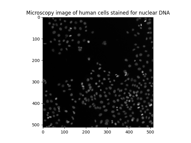
我们可以在黑暗的背景上看到许多细胞核。它们大多是光滑的，呈椭圆形。然而，我们可以辨别出一些与原子核经历的 mitosis (细胞分裂)。

另一种可视化灰度图像的方法是绘制等高线：

fig, ax = plt.subplots(figsize=(5, 5))
qcs = ax.contour(image, origin='image')
ax.set_title('Contour plot of the same raw image')
plt.show()

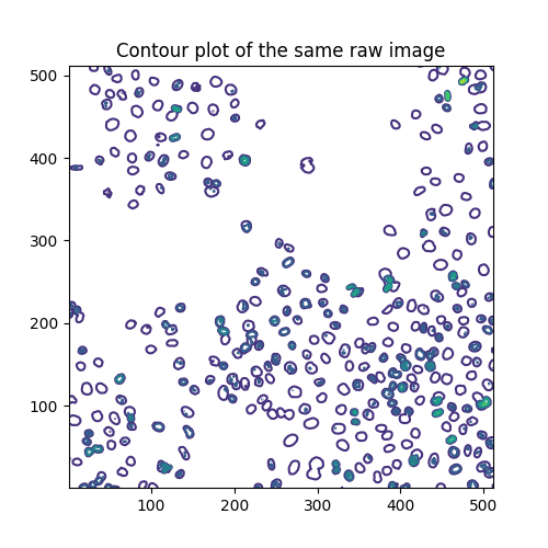
等高线是在以下标高绘制的：

qcs.levels

输出：

array([  0.,  40.,  80., 120., 160., 200., 240., 280.])

每个级别分别具有以下分段数：

[len(seg) for seg in qcs.allsegs]

输出：

[0, 320, 270, 48, 19, 3, 1, 0]

估计有丝分裂指数

细胞生物学使用 mitotic index 以量化细胞分裂，从而量化细胞增殖。根据定义，它是处于有丝分裂中的细胞占细胞总数的比率。为了分析上面的图像，我们对两个阈值感兴趣：一个是将核与背景分开，另一个是将分裂的核(亮点)与未分割的核分开。为了分离这三类不同的像素，我们求助于 多大津阈值 。

thresholds = filters.threshold_multiotsu(image, classes=3)
regions = np.digitize(image, bins=thresholds)

fig, ax = plt.subplots(ncols=2, figsize=(10, 5))
ax[0].imshow(image)
ax[0].set_title('Original')
ax[0].axis('off')
ax[1].imshow(regions)
ax[1].set_title('Multi-Otsu thresholding')
ax[1].axis('off')
plt.show()

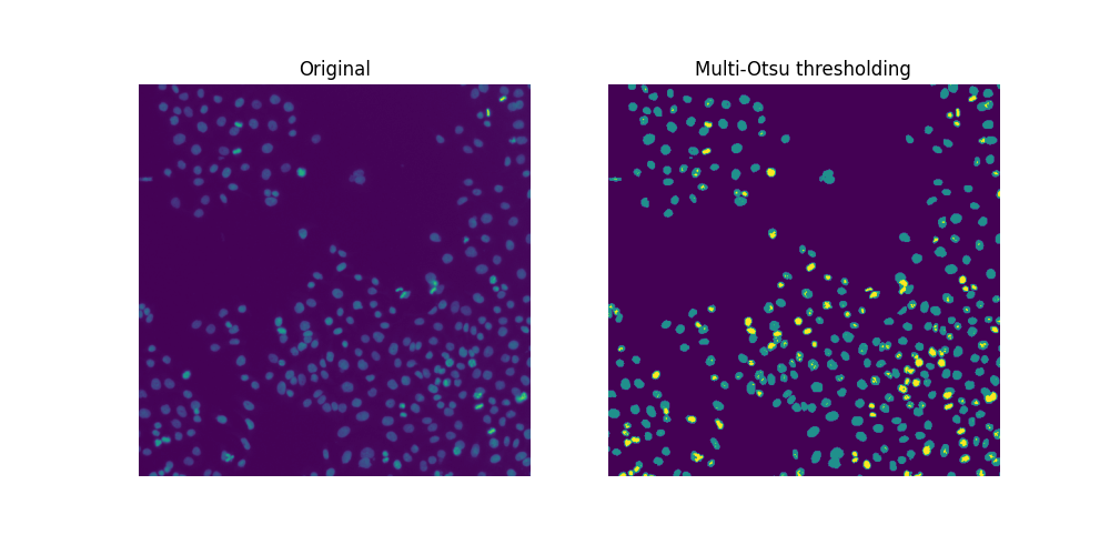
由于存在重叠的核团，阈值分割不足以分割所有的核团。如果是，我们可以很容易地计算出这个样本的有丝分裂指数：

cells = image > thresholds[0]
dividing = image > thresholds[1]
labeled_cells = measure.label(cells)
labeled_dividing = measure.label(dividing)
naive_mi = labeled_dividing.max() / labeled_cells.max()
print(naive_mi)

输出：

0.7847222222222222

哇，这不可能！分裂核数

print(labeled_dividing.max())

输出：

226

被高估了，而细胞总数

print(labeled_cells.max())

输出：

288

被低估了。

fig, ax = plt.subplots(ncols=3, figsize=(15, 5))
ax[0].imshow(image)
ax[0].set_title('Original')
ax[0].axis('off')
ax[2].imshow(cells)
ax[2].set_title('All nuclei?')
ax[2].axis('off')
ax[1].imshow(dividing)
ax[1].set_title('Dividing nuclei?')
ax[1].axis('off')
plt.show()

对分裂核进行计数

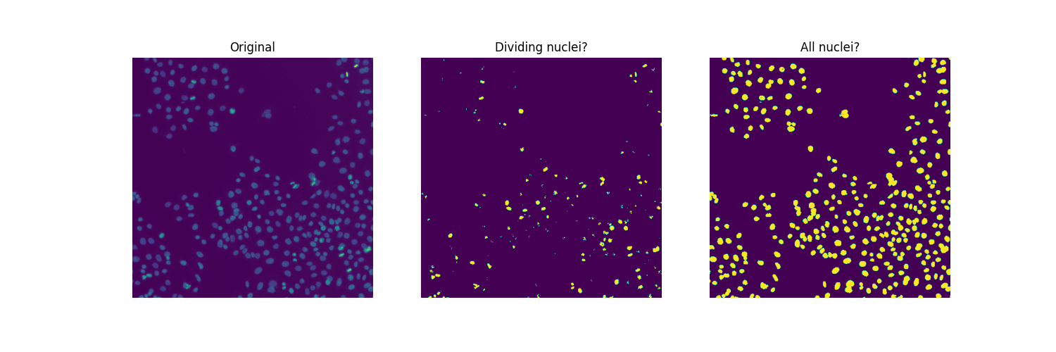
显然，并不是中间图中的所有连通区域都在划分原子核。一方面，第二个阈值(的值 thresholds[1] )似乎太低，无法将与划分核相对应的那些非常亮的区域与许多核中存在的相对亮的像素分开。另一方面，我们想要一个更平滑的图像，去除小的虚假物体，并可能合并相邻物体的集群(其中一些可能对应于从一个细胞分裂中出现的两个核)。在某种程度上，我们面临的分裂细胞核的分割挑战与(接触)细胞的分割挑战相反。

为了找到合适的阈值和过滤参数的值，我们通过视觉和手动两种方法进行。

higher_threshold = 125
dividing = image > higher_threshold

smoother_dividing = filters.rank.mean(util.img_as_ubyte(dividing),
                                      morphology.disk(4))

binary_smoother_dividing = smoother_dividing > 20

fig, ax = plt.subplots(figsize=(5, 5))
ax.imshow(binary_smoother_dividing)
ax.set_title('Dividing nuclei')
ax.axis('off')
plt.show()

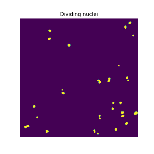
我们只剩下

cleaned_dividing = measure.label(binary_smoother_dividing)
print(cleaned_dividing.max())

输出：

29

在这个样本中划分出了原子核。

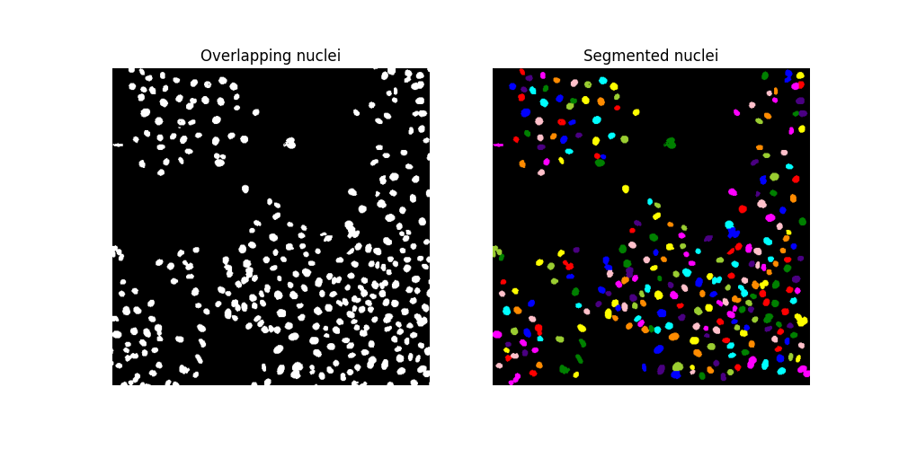
节段性核

为了分离重叠的原子核，我们求助于 分水岭分割 。为了便于可视化分割，我们使用 color.label2rgb 函数，并使用参数指定背景标签 bg_label=0 。

distance = ndi.distance_transform_edt(cells)

local_max_coords = feature.peak_local_max(distance, min_distance=7)
local_max_mask = np.zeros(distance.shape, dtype=bool)
local_max_mask[tuple(local_max_coords.T)] = True
markers = measure.label(local_max_mask)

segmented_cells = segmentation.watershed(-distance, markers, mask=cells)

fig, ax = plt.subplots(ncols=2, figsize=(10, 5))
ax[0].imshow(cells, cmap='gray')
ax[0].set_title('Overlapping nuclei')
ax[0].axis('off')
ax[1].imshow(color.label2rgb(segmented_cells, bg_label=0))
ax[1].set_title('Segmented nuclei')
ax[1].axis('off')
plt.show()

此外，我们还可以使用函数 color.label2rgb 使用透明度(Alpha参数)使用分割结果覆盖原始图像。

color_labels = color.label2rgb(segmented_cells, image, alpha=0.4, bg_label=0)

fig, ax = plt.subplots(figsize=(5, 5))
ax.imshow(color_labels)
ax.set_title('Segmentation result over raw image')
plt.show()

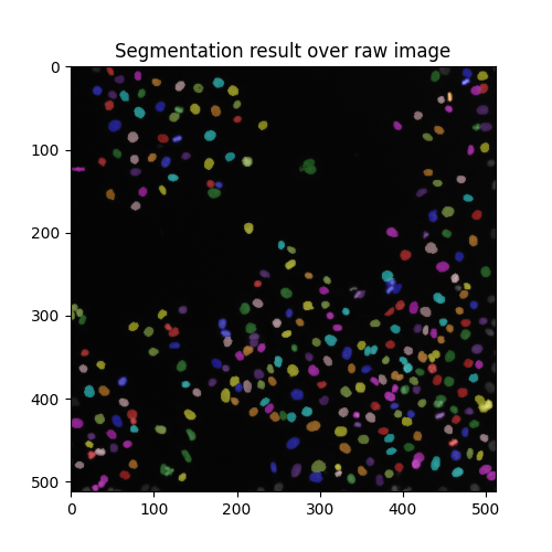
最后，我们发现总共有几个

print(segmented_cells.max())

输出：

286

这个样本中的细胞。因此，我们估计有丝分裂指数为：

print(cleaned_dividing.max() / segmented_cells.max())

输出：

0.10139860139860139