次轴

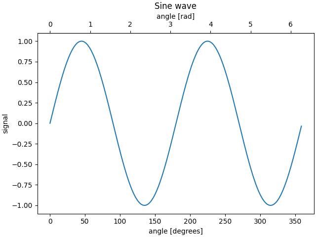
有时我们希望在绘图上有一个辅助轴，例如在同一个绘图上将弧度转换为度数。我们可以通过使只有一个轴可见的子轴通过 axes.Axes.secondary_xaxis 和 axes.Axes.secondary_yaxis . 通过将元组中的正向和反向转换函数提供给 functions kwarg：

import matplotlib.pyplot as plt
import numpy as np
import datetime
import matplotlib.dates as mdates
from matplotlib.ticker import AutoMinorLocator

fig, ax = plt.subplots(constrained_layout=True)
x = np.arange(0, 360, 1)
y = np.sin(2 * x * np.pi / 180)
ax.plot(x, y)
ax.set_xlabel('angle [degrees]')
ax.set_ylabel('signal')
ax.set_title('Sine wave')


def deg2rad(x):
    return x * np.pi / 180


def rad2deg(x):
    return x * 180 / np.pi


secax = ax.secondary_xaxis('top', functions=(deg2rad, rad2deg))
secax.set_xlabel('angle [rad]')
plt.show()

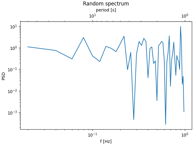
这里是在对数尺度下从波数转换为波长的例子。

注解

在这种情况下，父级的XScale是对数的，因此子级也被设为对数。

fig, ax = plt.subplots(constrained_layout=True)
x = np.arange(0.02, 1, 0.02)
np.random.seed(19680801)
y = np.random.randn(len(x)) ** 2
ax.loglog(x, y)
ax.set_xlabel('f [Hz]')
ax.set_ylabel('PSD')
ax.set_title('Random spectrum')


def forward(x):
    return 1 / x


def inverse(x):
    return 1 / x


secax = ax.secondary_xaxis('top', functions=(forward, inverse))
secax.set_xlabel('period [s]')
plt.show()

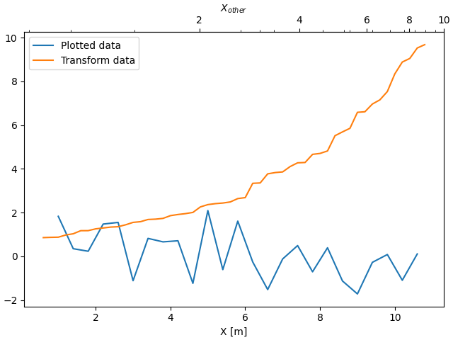
有时，我们希望将转换中的轴关联起来，该转换是从数据中特设的，并且是根据经验推导出来的。在这种情况下，我们可以将正向和反向变换函数设置为从一个数据集到另一个数据集的线性插值。

fig, ax = plt.subplots(constrained_layout=True)
xdata = np.arange(1, 11, 0.4)
ydata = np.random.randn(len(xdata))
ax.plot(xdata, ydata, label='Plotted data')

xold = np.arange(0, 11, 0.2)
# fake data set relating x coordinate to another data-derived coordinate.
# xnew must be monotonic, so we sort...
xnew = np.sort(10 * np.exp(-xold / 4) + np.random.randn(len(xold)) / 3)

ax.plot(xold[3:], xnew[3:], label='Transform data')
ax.set_xlabel('X [m]')
ax.legend()


def forward(x):
    return np.interp(x, xold, xnew)


def inverse(x):
    return np.interp(x, xnew, xold)


secax = ax.secondary_xaxis('top', functions=(forward, inverse))
secax.xaxis.set_minor_locator(AutoMinorLocator())
secax.set_xlabel('$X_{other}$')

plt.show()

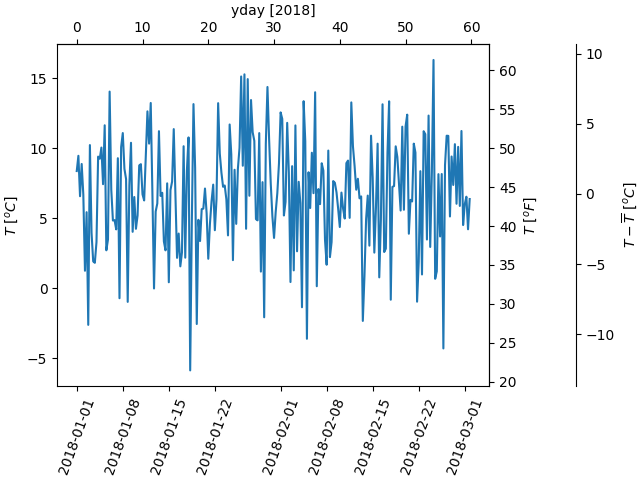
最后一个例子是np.datetime64在x轴上从摄氏度到华氏度，在y轴上从摄氏度到华氏度。注意添加了第三个y轴，并且可以使用float作为location参数来放置它

dates = [datetime.datetime(2018, 1, 1) + datetime.timedelta(hours=k * 6)
         for k in range(240)]
temperature = np.random.randn(len(dates)) * 4 + 6.7
fig, ax = plt.subplots(constrained_layout=True)

ax.plot(dates, temperature)
ax.set_ylabel(r'$T\ [^oC]$')
plt.xticks(rotation=70)


def date2yday(x):
    """Convert matplotlib datenum to days since 2018-01-01."""
    y = x - mdates.date2num(datetime.datetime(2018, 1, 1))
    return y


def yday2date(x):
    """Return a matplotlib datenum for *x* days after 2018-01-01."""
    y = x + mdates.date2num(datetime.datetime(2018, 1, 1))
    return y


secax_x = ax.secondary_xaxis('top', functions=(date2yday, yday2date))
secax_x.set_xlabel('yday [2018]')


def celsius_to_fahrenheit(x):
    return x * 1.8 + 32


def fahrenheit_to_celsius(x):
    return (x - 32) / 1.8


secax_y = ax.secondary_yaxis(
    'right', functions=(celsius_to_fahrenheit, fahrenheit_to_celsius))
secax_y.set_ylabel(r'$T\ [^oF]$')


def celsius_to_anomaly(x):
    return (x - np.mean(temperature))


def anomaly_to_celsius(x):
    return (x + np.mean(temperature))


# use of a float for the position:
secax_y2 = ax.secondary_yaxis(
    1.2, functions=(celsius_to_anomaly, anomaly_to_celsius))
secax_y2.set_ylabel(r'$T - \overline{T}\ [^oC]$')


plt.show()

---

工具书类

本例中显示了以下函数和方法的使用：

import matplotlib

matplotlib.axes.Axes.secondary_xaxis
matplotlib.axes.Axes.secondary_yaxis

出：

<function Axes.secondary_yaxis at 0x7faa00db2730>